
Turning off subtotals for a field in Excel
If you kick things up a notch and add a third field to the row or column area, Excel displays two sets of subtotals: one for the second (middle) field and one for the first (outer) field. And for every extra field you add to the row or column area, Excel mindlessly adds yet another set of subtotals.An Excel PivotTable displaying two or more sets of subtotals in one area is no picnic to read. Do yourself a favor and reduce the complexity of the PivotTable layout by turning off the subtotals for one or more of the fields. Here’s how:
- Select any cell in the field you want to work with.
- Choose Analyze → Field Settings.
The Field Settings dialog box appears with the Subtotals & Filters tab displayed.
- In the Subtotals group, select the None radio button.
Alternatively, right-click any cell in the field and then deselect the Subtotal “Field” command, where Field is the name of the field.
- Click OK.
Excel hides the field’s subtotals.
Displaying multiple subtotals for a field in Excel
When you add a second field to the row or column area, Excel displays a subtotal for each item in the outer field, and that subtotal uses the Sum calculation. If you prefer to see the Average for each item or the Count, you can change the field’s summary calculation.However, a common data analysis task is to view items from several different points of view. That is, you study the results by eyeballing not just a single summary calculation, but several: Sum, Average, Count, Max, Min, and so on.
That’s awesome of you, but it’s not all that easy to switch from one summary calculation to another. To avoid this problem, Excel enables you to view multiple subtotals for each field, with each subtotal using a different summary calculation. It’s true. You can use as many of Excel’s 11 built-in summary calculations as you need. That said, however, it’s useful to know that using StdDev and StDevp at the same time doesn't make sense, because the former is for sample data and the latter is for population data. The same is true for the Var and Varp calculations.
Okay, here are the steps to follow to add multiple subtotals to a field in Excel:
- Select any cell in the field you want to mess with.
- Choose Analyze →Field Settings.
The Field Settings dialog box appears with the Subtotals & Filters tab displayed.
- In the Subtotals group, select the Custom radio button.
- In the list that appears below the Custom options, select each calculation that you want to appear as a subtotal.
Alternatively, right-click any cell in the field and then deselect the Subtotal “Field” command, where Field is the name of the field.
- Click OK.
Excel recalculates the PivotTable to show the subtotals you selected. The following image shows an example PivotTable showing the Sum, Average, Max, and Min subtotals.
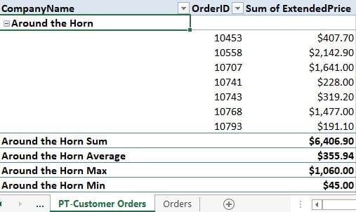 A PivotTable with multiple subtotals.