The COUNT function only counts the number of cells that contain numerical values in a range. It will completely ignore blank cells and any cells within the range that don’t contain numerical values, such as text. For this reason, the COUNT function is used only if you specifically want to count the numbers only.
Calculating a full-year projection using COUNT functions
Let’s try calculating a full-year projection using the COUNT and COUNTA functions. For example, say you have only ten months of data, and you want to do a full-year projection for your monthly budget meeting. You can calculate how many months’ worth of data you have by using the formula =COUNT(B2:B13), which will give you the correct number of elapsed months (10).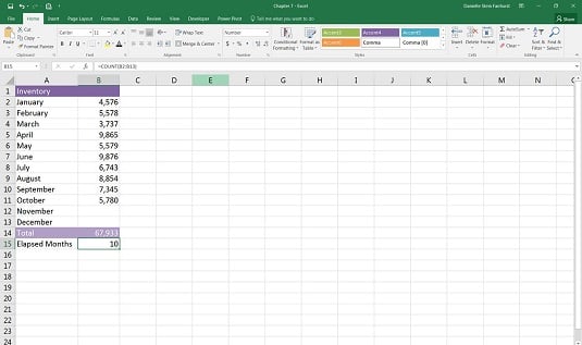
To insert the function, you can either type out the formula in cell B15, or select Count Numbers from the drop-down list next AutoSum button on the Home tab or the Formulas tab.
Note that the COUNTA function would work just as well in this case, but you particularly want to count only numbers, so you should stick with the COUNT function this time.Try adding a number in for November, and notice that the elapsed months changes to 11. This is exactly what you want to happen because it will automatically update whenever you add new data.
In cell B16, calculate the average monthly amount of inventory for the months that have already elapsed. You can do this using the formula =B14/B15. Then you can convert this number to an annual amount by multiplying it by 12. So, the entire formula is =B14/B15*12, which yields the result of 81,520.
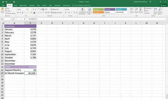
You can achieve exactly the same result using the formula =AVERAGE(B2:B13)*12. Which function you choose to use in your model is up to you, but the AVERAGE function does not require you to calculate the elapsed number of months as shown in row 15 in the image above. It’s a good idea to see the number of months shown on the page so you can make sure the formula is working correctly.
Calculating headcount costs with the COUNT function
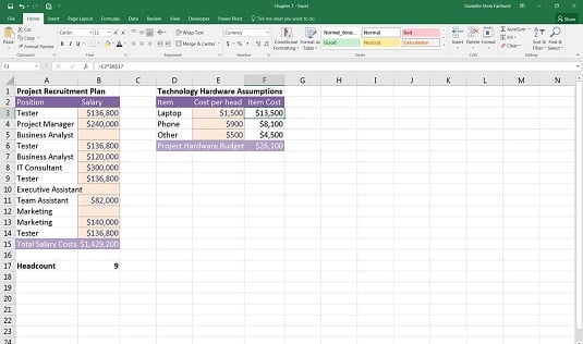
Let’s take a look at another example where the COUNT function can be useful. I often use the COUNT function to calculate headcount in a budget as it’s entered. For a practical example of how to use the COUNT function as part of a financial model, follow these steps:- Download File 0701.xlsx, open it, and select the tab labeled 7-15 or enter and format the data.
- In cell B17, enter the formula =COUNT(B3:B14) to count the number of staff in the budget.
You get the result of 9.
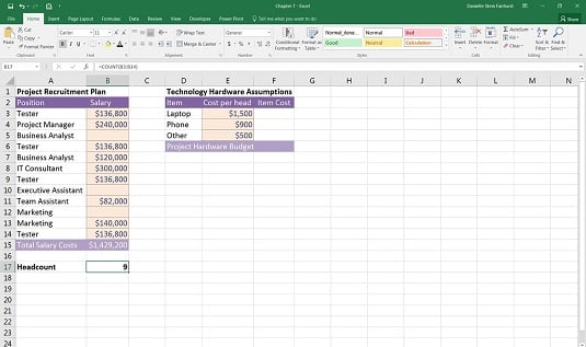
Again, the COUNTA function would’ve worked in this situation, but I specifically wanted to add up only the number of staff for which I have a budget.
Try entering TBD in one of the blank cells in the range. What happens? The COUNT function doesn’t change its value because it only counts cells with numerical values. Try using the COUNTA function instead (with TBD still in place in one of the formerly blank cells). The result changes from 9 to 10, which may or may not be what you want to happen.After you’ve calculated the headcount, you can incorporate this information into your technology budget. Each of the costs in the budget is a variable cost driven by headcount. Follow these steps:
- In cell F3, enter the formula =E3*B17.
This formula automatically calculates the total cost of all laptops based on the headcount numbers.
Because you want to copy this formula down, you need to anchor the cell reference to the headcount.
- Change the formula to =E3*$B$17 by using the F4 shortcut key or typing in the dollar signs manually.
- Copy the formula down the range, and add a total at the bottom.The completed budget.