
The most popular of the Excel 2016 lookup functions are HLOOKUP (for Horizontal Lookup) and VLOOKUP (for Vertical Lookup) functions. These functions are located on the Lookup & Reference drop-down menu on the Formulas tab of the Ribbon as well as in the Lookup & Reference category in the Insert Function dialog box. They are part of a powerful group of functions that can return values by looking them up in data tables.
The VLOOKUP function searches vertically (from top to bottom) the leftmost column of a Lookup table until the program locates a value that matches or exceeds the one you are looking up. The HLOOKUP function searches horizontally (from left to right) the topmost row of a Lookup table until it locates a value that matches or exceeds the one that you're looking up.
The VLOOKUP function uses the following syntax:
VLOOKUP(lookup_value,table_array,col_index_num,[range_lookup])
The HLOOKUP function follows the nearly identical syntax:
HLOOKUP(lookup_value,table_array,row_index_num,[range_lookup])
In both functions, the lookup_value argument is the value that you want to look up in the Lookup table, and table_array is the cell range or name of the Lookup table that contains both the value to look up and the related value to return.
The col_index_num argument designates the column of the lookup table containing the values that are returned by the VLOOKUP function based on matching the value of the lookup_value argument against those in the table_array argument. You determine the col_index_num argument counting how many columns this column is over to the right from the first column of the vertical Lookup table, and you include the first column of the Lookup table in this count.
The row_index_num argument designates the row containing the values are returned by the HLOOKUP function in a horizontal table. You determine the row_index_num argument by counting how many rows down this row is from the top row of the horizontal Lookup table. Again, you include the top row of the Lookup table in this count.
When entering the col_index_num or row_index_num arguments in the VLOOKUP and HLOOKUP functions, the value you entercannot exceed the total number of columns or rows in the Lookup table.
The optional range_lookup argument in both the VLOOKUP and the HLOOKUP functions is the logical TRUE or FALSE that specifies whether you want Excel to find an exact or approximate match for the lookup_value in the table_array. When you specify TRUE or omit the range_lookup argument in the VLOOKUP or HLOOKUP function, Excel finds an approximate match. When you specify FALSE as the range_lookup argument, Excel finds only exact matches.
Finding approximate matches pertains only when you're looking up numeric entries (rather than text) in the first column or row of the vertical or horizontal Lookup table. When Excel doesn't find an exact match in this Lookup column or row, it locates the next highest value that doesn't exceed the lookup_value argument and then returns the value in the column or row designated by the col_index_num or row_index_num arguments.
When using the VLOOKUP and HLOOKUP functions, the text or numeric entries in the Lookup column or row (that is, the leftmost column of a vertical Lookup table or the top row of a horizontal Lookup table) must be unique. These entries must also be arranged or sorted in ascending order; that is, alphabetical order for text entries, and lowest-to-highest order for numeric entries.
The figure shows an example of using the VLOOKUP function to return either a 15% or 20% tip from a tip table, depending on the pretax total of the check. Cell F3 contains the VLOOKUP function:
=VLOOKUP(Pretax_Total,Tip_Table,IF(Tip_Percentage=0.15,2,3))
This formula returns the amount of the tip based on the tip percentage in cell F1 and the pretax amount of the check in cell F2.
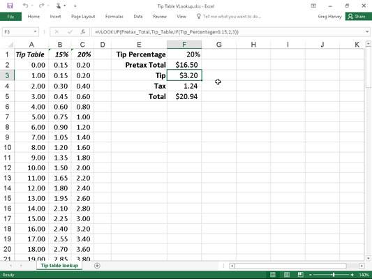
To use this tip table, enter the percentage of the tip (15% or 20%) in cell F1 (named Tip_Percentage) and the amount of the check before tax in cell F2 (named Pretax_Total). Excel then looks up the value that you enter in the Pretax_Total cell in the first column of the Lookup table, which includes the cell range A2:C101 and is named Tip_Table.
Excel then moves down the values in the first column of Tip_Table until it finds a match, whereupon the program uses the col_index_num argument in the VLOOKUP function to determine which tip amount from that row of the table to return to cell F3. If Excel finds that the value entered in the Pretax_Total cell ($16.50 in this example) doesn't exactly match one of the values in the first column of Tip_Table, the program continues to search down the comparison range until it encounters the first value that exceeds the pretax total (17.00 in cell A19 in this example). Excel then moves back up to the previous row in the table and returns the value in the column that matches the col_index_num argument of the VLOOKUP function. (This is because the optional range_lookup argument has been omitted from the function.)
Note that the tip table example in the figure uses an IF function to determine the col_index_num argument for the VLOOKUP function in cell F3. The IF function determines the column number to be used in the tip table by matching the percentage entered in Tip_Percentage (cell F1) with 0.15. If they match, the function returns 2 as the col_index_num argument and the VLOOKUP function returns a value from the second column (the 15% column B) in the Tip_Table range. Otherwise, the IF function returns 3 as the col_index_num argument and the VLOOKUP function returns a value from the third column (the 20% column C) in the Tip_Table range.
The following figure shows an example that uses the HLOOKUP function to look up the price of each bakery item stored in a separate price Lookup table and then to return that price to the Price/Doz column of the Daily Sales list. Cell F3 contains the original formula with the HLOOKUP function that is then copied down column F:
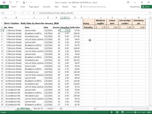
=HLOOKUP(item,Price_table,2,FALSE)
In this HLOOKUP function, the range name Item that's given to the Item column in the range C3:C62 is defined as the lookup_value argument and the cell range name Price table that's given to the cell range I1:M2 is the table_array argument. The row_index_num argument is 2 because you want Excel to return the prices in the second row of the Prices Lookup table, and the optional range_lookup argument is FALSE because the item name in the Daily Sales list must match exactly the item name in the Prices Lookup table.
By having the HLOOKUP function use the Price table range to input the price per dozen for each bakery goods item in the Daily Sales list, you make it a very simple matter to update any of the sales in the list. All you have to do is change its Price/Doz cost in this range, and the HLOOKUP function immediately updates the new price in the Daily Sales list wherever the item is sold.