Excel 2013’s Scenario Manager option on the What-If Analysis button’s drop-down menu on the Data tab of the Ribbon enables you to create and save sets of different input values that produce different calculated results, named scenarios. Because these scenarios are saved as part of the workbook, you can use their values to play what-if simply by opening the Scenario Manager and having Excel show the scenario in the worksheet.
After setting up the various scenarios for a spreadsheet, you can also have Excel create a summary report that shows both the input values used in each scenario as well as the results they produce in your formula.
How to set up the various scenarios in Excel 2013
The key to creating the various scenarios for a table is to identify the various cells in the data whose values can vary in each scenario. You then select these cells (known as changing cells) in the worksheet before you open the Scenario Manager dialog box by clicking Data→What-If Analysis→Scenario Manager on the Ribbon or by pressing Alt+AWS.
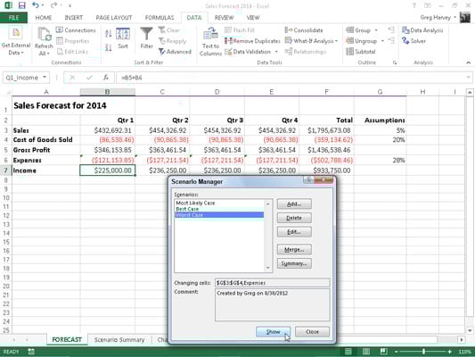
Below, you see the Sales Forecast 2014 table after selecting the three changing cells in the worksheet — H3 named Sales_Growth, H4 named COGS (Cost of Goods Sold), and H6 named Expenses — and then opening the Scenario Manager dialog box (Alt+AWS).
Let’s create three scenarios using the following sets of values for the three changing cells:
Most Likely Case where the Sales_Growth percentage is 5%, COGS is 20%, and Expenses is 28%
Best Case where the Sales_Growth percentage is 8%, COGS is 18%, and Expenses is 20%
Worst Case where the Sales_Growth percentage is 2%, COGS is 25%, and Expenses is 35%
To create the first scenario, click the Add button in the Scenario Manager dialog box to open the Add Scenario dialog box, enter Most Likely Case in the Scenario Name box, and then click OK. (Remember that the three cells currently selected in the worksheet, H3, H4, and H6, are already listed in the Changing Cells text box of this dialog box.)
Excel then displays the Scenario Values dialog box where you accept the following values already entered in each of the three text boxes (from the Sales Forecast 2014 table), Sales_Growth, COGS, and Expenses, before clicking its Add button:
0.05 in the Sales_Growth text box
0.2 in COGS text box
0.28 in the Expenses text box
Always assign range names to your changing cells before you begin creating the various scenarios that use them. That way, Excel always displays the cells’ range names rather than their addresses in the Scenario Values dialog box.
After clicking the Add button, Excel redisplays the Add Scenario dialog box where you enter Best Case in the Scenario Name box and the following values in the Scenario Values dialog box:
0.08 in the Sales_Growth text box
0.18 in the COGS text box
0.20 in the Expenses text box
After making these changes, click the Add button again. Doing this opens the Add Scenario dialog box where you enter Worst Case as the scenario name and the following scenario values:
0.02 in the Sales_Growth text box
0.25 in the COGS text box
0.35 in the Expenses text box
Because this is the last scenario that you want to add, then click the OK button instead of Add. Doing this opens the Scenario Manager dialog box again, this time displaying the names of all three scenarios — Most Likely Case, Best Case, and Worst Case — in its Scenarios list box.
To have Excel plug the changing values assigned to any of these three scenarios into the Sales Forecast 2014 table, click the scenario name in this list box followed by the Show button.
After adding the various scenarios for a table in your spreadsheet, don’t forget to save the workbook after closing the Scenario Manager dialog box. That way, you’ll have access to the various scenarios each time you open the workbook in Excel simply by opening the Scenario Manager, selecting the scenario name, and clicking the Show button.
How to produce an Excel 2013 summary report
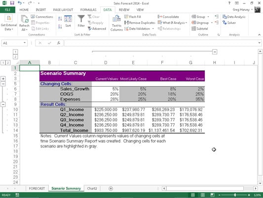
After adding your scenarios to a table in a spreadsheet, you can have Excel produce a summary report. This report displays the changing and resulting values for not only all the scenarios you’ve defined, but also the current values that are entered into the changing cells in the worksheet table at the time you generate the report.
To produce a summary report, open the Scenario Manager dialog box (Data→What-If Analysis→Scenario Manager or Alt+AWS) and then click the Summary button to open the Scenario Summary dialog box.
This dialog box gives you a choice between creating a (static) Scenario Summary (the default) and a (dynamic) Scenario PivotTable Report. You can also modify the range of cells in the table that is included in the Result Cells section of the summary report by adjusting the cell range in the Result Cells text box before you click OK to generate the report.
After you click OK, Excel creates the summary report for the changing values in all the scenarios (and the current worksheet) along with the calculated values in the Result Cells on a new worksheet (named Scenario Summary). You can then rename and reposition the Scenario Summary worksheet before you save it as part of the workbook file.