You use the Excel 2016 ROUND function found on the Math & Trig command button's drop-down menu to round up or down fractional values in the worksheet as you might when working with financial spreadsheets that need to show monetary values only to the nearest dollar.
Unlike when applying a number format to a cell, which affects only the number's display, the ROUND function actually changes the way Excel stores the number in the cell that contains the function. ROUND uses the following syntax:
ROUND(number,num_digits)
In this function, the number argument is the value that you want to round off, and num_digits is the number of digits to which you want the number rounded. If you enter 0 (zero) as the num_digits argument, Excel rounds the number to the nearest integer. If you make the num_digits argument a positive value, Excel rounds the number to the specified number of decimal places. If you enter the num_digits argument as a negative number, Excel rounds the number to the left of the decimal point.
Instead of the ROUND function, you can use the ROUNDUP or ROUNDDOWN function. Both ROUNDUP and ROUNDDOWN take the same number and num_digits arguments as the ROUND function. The difference is that the ROUNDUP function always rounds up the value specified by the number argument, whereas the ROUNDDOWN function always rounds the value down.
The figure illustrates the use of the ROUND, ROUNDUP, and ROUNDDOWN functions in rounding off the value of the mathematical constant pi. In cell A3, the value of this constant (with just nine places of nonrepeating fraction displayed when the column is widened) is entered into this cell, using Excel's PI function in the following formula:
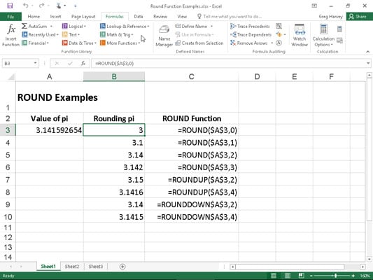
=PI()
Then the ROUND, ROUNDUP, and ROUNDDOWN functions were used in the cell range B3 through B10 to round this number up and down to various decimal places.
Cell B3, the first cell that uses one of the ROUND functions to round off the value of pi, rounds this value to 3 because 0 (zero) is used as the num_digits argument of its ROUND function (causing Excel to round the value to the nearest whole number).
In the figure, note the difference between using the ROUND and ROUNDUP functions both with 2 as their num_digits arguments in cells B5 and B7, respectively. In cell B5, Excel rounds the value of pi off to 3.14, whereas in cell B7, the program rounds its value up to 3.15. Note that using the ROUNDDOWN function with 2 as its num_digits argument yields the same result, 3.14, as does using the ROUND function with 2 as its second argument.
The whole number and nothing but the whole number
You can also use the INT (for Integer) and TRUNC (for Truncate) functions on the Math & Trig command button's drop-down menu to round off values in your spreadsheets. You use these functions only when you don't care about all or part of the fractional portion of the value. When you use the INT function, which requires only a single number argument, Excel rounds the value down to the nearest integer (whole number). For example, cell A3 contains the value of pi, as shown in the figure, and you enter the following INT function formula in the worksheet:
=INT(A3)
Excel returns the value 3 to the cell, the same as when you use 0 (zero) as the num_digits argument of the ROUND function in cell B3.
The TRUNC function uses the same number and num_digits arguments as the ROUND, ROUNDUP, and ROUNDDOWN functions, except that in the TRUNC function, the num_digits argument is purely optional. This argument is required in the ROUND, ROUNDUP, and ROUNDDOWN functions.
The TRUNC function doesn't round off the number in question; it simply truncates the number to the nearest integer by removing the fractional part of the number. However, if you specify a num_digits argument, Excel uses that value to determine the precision of the truncation. So, going back to the example illustrated in Figure 5-1, if you enter the following TRUNC function, omitting the optional num_digits argument as in
=TRUNC($A$3)
Excel returns 3 to the cell just like the formula =ROUND($A$3,0) does in cell B3. However, if you modify this TRUNC function by using 2 as its num_digits argument, as in
=TRUNC($A$3,2)
Excel then returns 3.14 (by cutting rest of the fraction) just as the formula =ROUND($A$3,2) does in cell B5.
The only time you notice a difference between the INT and TRUNC functions is when you use them with negative numbers. For example, if you use the TRUNC function to truncate the value –5.4 in the following formula:
=TRUNC(–5.4)
Excel returns –5 to the cell. If, however, you use the INT function with the same negative value, as in
=INT(–5.4)
Excel returns –6 to the cell. This is because the INT function rounds numbers down to the nearest integer using the fractional part of the number.
Let's call it even or odd
Excel's EVEN and ODD functions on the Math & Trig command button's drop-down menu also round off numbers. The EVEN function rounds the value specified as its number argument up to the nearest even integer. The ODD function, of course, does just the opposite: rounding the value up to the nearest odd integer. So, for example, if cell C18 in a worksheet contains the value 345.25 and you use the EVEN function in the following formula:
=EVEN(C18)
Excel rounds the value up to the next whole even number and returns 346 to the cell. If, however, you use the ODD function on this cell, as in
=ODD(C18)
Excel rounds the value up to the next odd whole number and returns 347 to the cell instead.
Building in a ceiling
The CEILING.MATH function on the Math & Trig command button's drop-down menu enables you to not only round up a number, but also set the multiple of significance to be used when doing the rounding. This function can be very useful when dealing with figures that need rounding to particular units.
For example, suppose that you're working on a worksheet that lists the retail prices for the various products that you sell, all based upon a particular markup over wholesale, and that many of these calculations result in many prices with cents below 50. If you don't want to have any prices in the list that aren't rounded to the nearest 50 cents or whole dollar, you can use the CEILING function to round up all these calculated retail prices to the nearest half dollar.
The CEILING.MATH function uses the following syntax:
CEILING.MATH(number,[significance],[mode])
The number argument specifies the number you want to round up and the optional significance argument specifies the multiple to which you want to round. (By default, the significance is +1 for positive numbers and –1 for negative numbers.) The optional mode argument comes into play only when dealing with negative numbers where the mode value indicates the direction toward (+1) or away (–1) from 0.
For the half-dollar example, suppose that you have the calculated number $12.35 in cell B3 and you enter the following formula in cell C3:
=CEILING.MATH(B3,0.5)
Excel then returns $12.50 to cell C3. Further, suppose that cell B4 contains the calculated value $13.67, and you copy this formula down to cell C4 so that it contains
=CEILING.MATH(B4,0.5)
Excel then returns $14.00 to that cell.
CEILING.MATH in Excel 2016 replaces the CEILING function supported in older versions of Excel. You can still use the CEILING function to round your values; just be aware that this function is no longer available on the Math & Trig drop-down menu on the FORMULAS tab of the Ribbon or in the Insert Function dialog box. This means that you have to type =cei directly into the cell to have the CEILING function appear in the function drop-down menu immediately below CEILING.MATH.