
You can use Excel 2016's handy Quick Analysis tool to quickly format your data as a new table. Simply select all the cells in the table, including the cells in the first row with the column headings. As soon as you do, the Quick Analysis tool appears in the lower-right corner of the cell selection (the outlined button with the lightning bolt striking the selected data icon).
When you click this tool, the Quick Analysis options palette appears with five tabs (Formatting, Charts, Totals, Tables, and Sparklines).
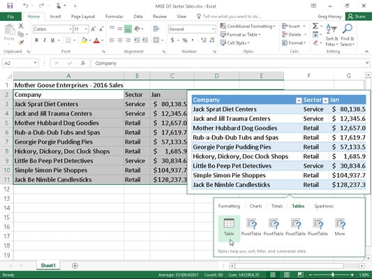
Click the Tables tab in the Quick Analysis tool's option palette to display its Table and Pivot Table buttons. When you highlight the Table button on the Tables tab, Excel's Live Preview shows you how the selected data will appear formatted as a table. (See the following figure.) To apply this previewed formatting and format the selected cell range as a table, you have only to click the Table button.
As soon as you click the Table button, the Quick Analysis options palette disappears and the Design contextual table appears on the Ribbon. You can then use its Table Styles drop-down gallery to select a different formatting style for your table. (The Tables button on the Quick Analysis tool's Tables tab offers only the one blue medium style shown in the Live Preview.)