
In a conventional formula in Excel 2016, you provide the raw data and Excel produces the results. With the Goal Seek command, you declare what you want the results to be and Excel tells you the raw data you need to produce those results.
The Goal Seek command is useful in analyses when you want the outcome to be a certain way and you need to know which raw numbers will produce the outcome that you want.
This figure shows a worksheet designed to find out the monthly payment on a mortgage. With the PMT function, the worksheet determines that the monthly payment on a $250,000 loan with an interest rate of 6.5 percent and to be paid over a 30-year period is $1,580.17.
Suppose, however, that the person who calculated this monthly payment determined that he or she could pay more than $1,580.17 per month? Suppose the person could pay $1,750 or $2,000 per month. Instead of an outcome of $1,580.17, the person wants to know how much he or she could borrow if monthly payments — the outcome of the formula — were increased to $1,750 or $2,000.
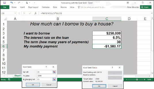
To make determinations such as these, you can use the Goal Seek command. This command lets you experiment with the arguments in a formula to achieve the results you want. In the case of the worksheet shown, you can use the Goal Seek command to change the argument in cell C3, the total amount you can borrow, given the outcome you want in cell C6, $1,750 or $2,000, the monthly payment on the total amount.
Follow these steps to use the Goal Seek command to change the inputs in a formula to achieve the results you want:
Select the cell with the formula whose arguments you want to experiment with.
On the Data tab, click the What-If Analysis button and choose Goal Seek on the drop-down list.
You see the Goal Seek dialog box shown. The address of the cell you selected in Step 1 appears in the Set Cell box.
In the To Value text box, enter the target results you want from the formula.
In the example, you enter -1750 or -2000, the monthly payment you can afford for the 30-year mortgage.
In the By Changing Cell text box, enter the address of the cell whose value is unknown.
To enter a cell address, go outside the Goal Seek dialog box and click a cell on your worksheet. You select the address of the cell that shows the total amount you want to borrow.
Click OK.
The Goal Seek Status dialog box appears, as shown. It lists the target value that you entered in Step 3.
Click OK.
On your worksheet, the cell with the argument you wanted to alter now shows the target you're seeking. In the case of the example worksheet in Figure 5-6, you can borrow $316,422 at 6.5 percent, not $250,000, by raising your monthly mortgage payments from $1,580.17 to $2,000.