
The Timeline slicer works in the same way a standard slicer does, in that it lets you filter a pivot table using a visual selection mechanism instead of the old Filter fields. The difference is the Timeline slicer is designed to work exclusively with date fields, providing an excellent visual method to filter and group the dates in your pivot table.
To create a Timeline slicer, your pivot table must contain a field where all data is formatted as a date. It's not enough to have a column of data that contains a few dates. All values in the date field must be a valid date and formatted as such.
To create a Timeline slicer, follow these steps:
Place the cursor anywhere inside the pivot table and then click the Analyze tab on the Ribbon.
Click the tab's Insert Timeline command, shown here.
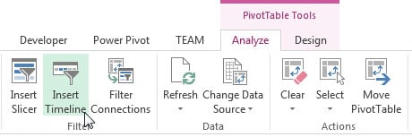 Inserting a Timeline slicer.
The Insert Timelines dialog box shown here appears, showing you all available date fields in the chosen pivot table.
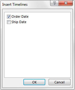 Select the date fields for which you want slicers created.
In the Insert Timelines dialog box, select the date fields for which you want to create the timeline.
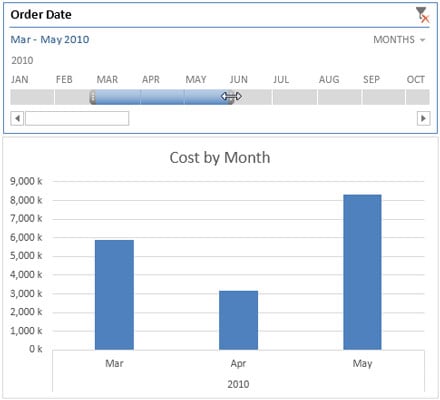
After your Timeline slicer is created, you can filter the data in the pivot table and pivot chart using this dynamic data selection mechanism. The following figure demonstrates how selecting Mar, Apr, and May in the Timeline slicer automatically filters the pivot chart.
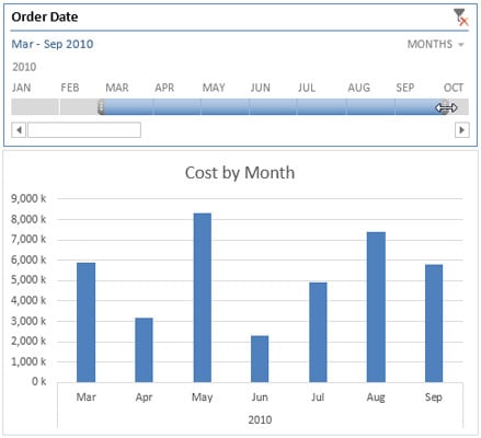
The following figure illustrates how you can expand the slicer range with the mouse to include a wider range of dates in your filtered numbers.
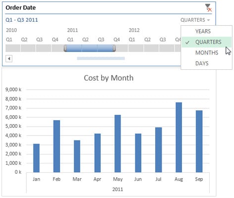
Want to quickly filter your pivot table by quarters? Well, that's easy with a Timeline slicer. Simply click the time period drop-down menu and select Quarters. As you can see, you can also switch to Years or Days, if needed.
Timeline slicers are not backward compatible: They are usable only in Excel 2013 and Excel 2016. If you open a workbook with Timeline slicers in Excel 2010 or previous versions, the Timeline slicers will be disabled.