
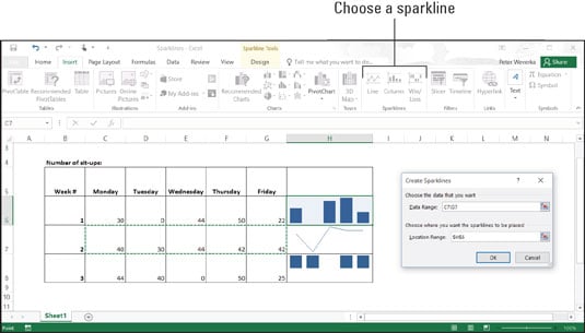
Maybe the easiest way to analyze information in an Excel 2016 worksheet is to see what the sparklines say. this figure shows examples of sparklines. In the form of a tiny line or bar chart, sparklines tell you about the data in a row or column.
Follow these steps to create a sparkline chart:
Select the cell where you want the chart to appear.
On the Insert tab, click the Line, Column, or Win/Loss button.
The Create Sparklines dialog box appears.
Drag in a row or column of your worksheet to select the cells with the data you want to analyze.
Click OK in the Create Sparklines dialog box.
To change the look of a sparkline chart, go to the (Sparkline Tools) Design tab. There you will find commands for changing the color of the line or bars, choosing a different sparkline type, and doing one or two other things to pass the time on a rainy day. Click the Clear button to remove a sparkline chart.
You can also create a sparkline chart with the Quick Analysis button. Drag over the cells with the data you want to analyze. When the Quick Analysis button appears, click it, choose Sparklines in the pop-up window, and then choose Line, Column, or Win/Loss.