How to Add Your Own Excel Formatting Rules Manually

You don't have to use one of the predefined scenarios offered by Excel. Excel gives you the flexibility to create your own formatting rules manually. Creating your own formatting rules helps you better control how cells are formatted and allows you to do things you wouldn't be able to do with the predefined scenarios.

For example, a useful conditional formatting rule is to tag all above-average values with a Check icon and all below-average values with an X icon. The figure demonstrates this rule.

With a custom formatting rule, you can tag the above-average values with a check mark and the below-average values with an X.

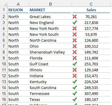
Although it's true that the Above Average and Below Average scenarios built into Excel allow you to format cell and font attributes, they don't enable the use of Icon Sets. You can imagine why Icon Sets would be better on a dashboard than simply color variances. Icons and shapes do a much better job of conveying your message, especially when the dashboard is printed in black-and-white.

To get started in creating your first custom formatting rule, go to the Create Rule by Hand tab, and then follow these steps:

1. Select the target range of cells to which you need to apply the conditional formatting, and select New Rule from the Conditional Formatting menu, as demonstrated.

   

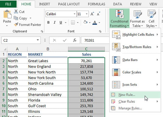   Select the target range and then select New Rule.

   This step opens the New Formatting Rule dialog box shown in the following figure.

   

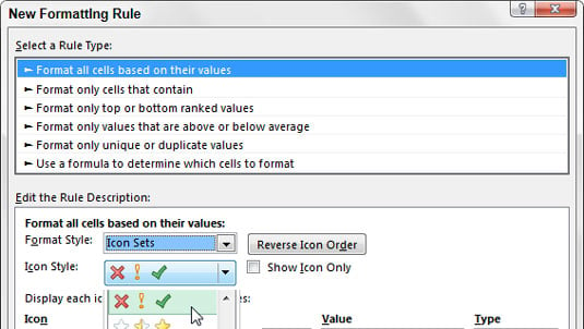   Select the Format All Cells Based on Their Values rule and then use the Format Style drop-down menu to switch to Icon Sets.

   Here's what each type does:

   • Format All Cells Based on Their Values: Measures the values in the selected range against each other. This selection is handy for finding general anomalies in your dataset.

   • Format Only Cells That Contain: Applies conditional formatting to those cells that meet specific criteria you define. This selection is perfect for comparing values against a defined benchmark.

   • Format Only Top or Bottom Ranked Values: Applies conditional formatting to those cells that are ranked in the top or bottom Nth number or percent of all values in the range.

   • Format Only Values That Are Above or Below Average: Applies conditional formatting to those values that are mathematically above or below the average of all values in the selected range.

   • Use a Formula to Determine Which Cells to Format: Evaluates values based on a formula you specify. If a particular value evaluates to true, the conditional formatting is applied to that cell. This selection is typically used when applying conditions based on the results of an advanced formula or mathematical operation.

   Data Bars, Color Scales, and Icon Sets can be used only with the Format All Cells Based on Their Values rule type.

2. Ensure that the Format All Cells Based on Their Values rule type is selected and then use the Format Style drop-down menu to switch to Icon Sets.

3. Click the Icon Style drop-down menu to select an Icon Set.

4. Change both Type drop-down menus to Formula.

5. In each Value box, enter =Average($C$2:$C$22).

   This step tells Excel that the value in each cell must be greater than the average of the entire dataset in order to get the Check icon.

   At this point, the dialog box looks similar to the one shown here.

   

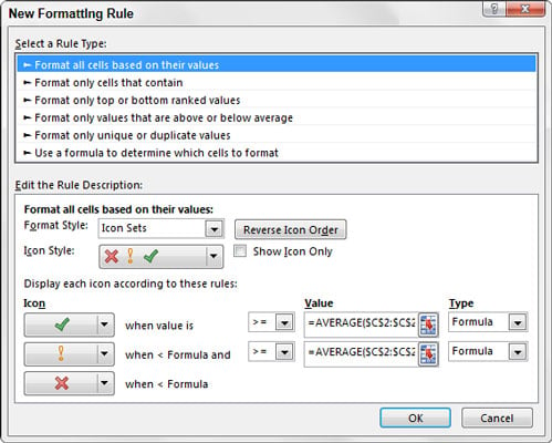   Change the Type drop-down boxes to Formula and enter the appropriate formulas in the Value boxes.

6. Click OK to apply your conditional formatting.

It's worth taking some time to understand how this conditional formatting rule works. Excel assesses every cell in the target range to see whether its contents match, in order (top box first), the logic in each Value box. If a cell contains a number or text that evaluates true to the first Value box, the first icon is applied and Excel moves on to the next cell in the range. If not, Excel continues down each Value box until one of them evaluates to true. If the cell being assessed does not fit any of the logic placed in the Value boxes, Excel automatically tags that cell with the last icon.

In this example, you want a cell to get a Check icon only if the value of the cell is greater than (or equal to) the average of the total values. Otherwise, you want Excel to skip directly to the X icon and apply the X.