Often, your customers want to look at clean, round numbers. Inundating a user with decimal values and unnecessary digits for the sake of precision can actually make your reports harder to read. For this reason, you may want to consider using Excel’s rounding functions.
This figure illustrates how the number 9.45 is affected by the use of the ROUND, ROUNDUP, and ROUNDDOWN functions.
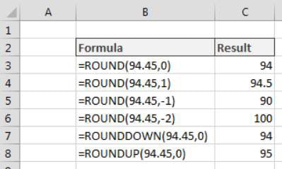
Excel’s ROUND function is used to round a given number to a specified number of digits. The ROUND function takes two arguments: the original value and the number of digits to round to.
Entering a 0 as the second argument tells Excel to remove all decimal places and round the integer portion of the number based on the first decimal place. For instance, this formula rounds to 94:
=ROUND(94.45,0)
Entering a 1 as the second argument tells Excel to round to one decimal based on the value of the second decimal place. For example, this formula rounds to 94.5:
=ROUND(94.45,1)
You can also enter a negative number as the second argument, telling Excel to round based on values to the left of the decimal point. The following formula, for example, returns 90:
=ROUND(94.45,-1)
You can force rounding in a particular direction using the ROUNDUP or ROUNDDOWN functions.
This ROUNDDOWN formula rounds 94.45 down to 94:
=ROUNDDOWN(94.45,0)
This ROUNDUP formula rounds 94.45 up to 95:
=ROUNDUP(94.45,0)
Rounding to the nearest penny in Excel
In some industries, it is common practice to round a dollar amount to the nearest penny. The figure demonstrates how rounding a dollar amount up or down to the nearest penny can affect the resulting number.
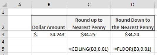
You can round to the nearest penny by using the CEILING or FLOOR functions.
The CEILING function rounds a number up to the nearest multiple of significance that you pass to it. This utility comes in handy when you need to override the standard rounding protocol with your own business rules. For instance, you can force Excel to round 123.222 to 124 by using the CEILING function with a significance of 1.
=CEILING(123.222,1)
So entering a .01 as the significance tells the CEILING function to round to the nearest penny.
If you wanted to round to the nearest nickel, you could use .05 as the significance. For instance, the following formula returns 123.15:
=CEILING(123.11,.05)
The FLOOR function works the same way except that it forces a rounding down to the nearest significance. The following example function rounds 123.19 down to the nearest nickel, giving 123.15 as the result:
=FLOOR(123.19,.05)
Rounding to significant digits in Excel
In some financial reports, figures are presented in significant digits. The idea is that when you’re dealing with numbers in the millions, you don’t need to inundate a report with superfluous numbers for the sake of showing precision down to the tens, hundreds, and thousands places.
For instance, instead of showing the number 883,788, you could choose to round the number to one significant digit. This would mean displaying the same number as 900,000. Rounding 883,788 to two significant digits would show the number as 880,000.
In essence, you’re deeming that a particular number’s place is significant enough to show. The rest of the number can be replaced with zeros. You might feel as though doing this could introduce problems, but when you’re dealing with large enough numbers, any number below a certain significance is inconsequential.
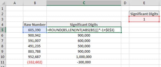
The following figure demonstrates how you can implement a formula that rounds numbers to a given number of significant digits.
You use Excel’s ROUND function to round a given number to a specified number of digits. The ROUND function takes two arguments: the original value and the number of digits to round to.
Entering a negative number as the second argument tells Excel to round based on significant digits to the left of the decimal point. The following formula, for example, returns 9500:
=ROUND(9489,-2)
Changing the significant digits argument to -3 returns a value of 9000.
=ROUND(B14,-3)
This works great, but what if you have numbers on differing scales? That is, what if some of your numbers are millions while others are hundreds of thousands? If you wanted to show them all with 1 significant digit, you would need to build a different ROUND function for each number to account for the differing significant digits argument that you would need for each type of number.
To help solve this issue, you can replace your hard-coded significant digits argument with a formula that calculates what that number should be.
Imagine that your number is -2330.45. You can use this formula as the significant digits argument in your ROUND function:
LEN(INT(ABS(-2330.45)))*-1+2
This formula first wraps your number in the ABS function, effectively removing any negative symbol that may exist. It then wraps that result in the INT function, stripping out any decimals that may exist. It then wraps that result in the LEN function to get a measure of how many characters are in the number without any decimals or negation symbols.
In this example, this part of the formula results in the number 4. If you take the number –2330.45 and strip away the decimals and negative symbol, you have four characters left.
This number is then multiplied by -1 to make it a negative number, and then added to the number of significant digits you are looking for. In this example, that calculation looks like this: 4 * –1 + 2 = –2.
Again, this formula will be used as the second argument for your ROUND function. Enter this formula into Excel and round the number to 2300 (2 significant digits):
=ROUND(-2330.45, LEN(INT(ABS(-2330.45)))*-1+2)
You can then replace this formula with cell references that point to the source number and cell that holds the number of desired significant digits.
=ROUND(B5,LEN(INT(ABS(B5)))*-1+$E$3)