Excel 2019 Formatting: Using the Format as Table Gallery

As soon as you click one of the table formatting thumbnails in this Table Styles gallery, Excel makes its best guess as to the cell range of the data table to apply it to (indicated by the marquee around its perimeter), and the Format As Table dialog box appears.

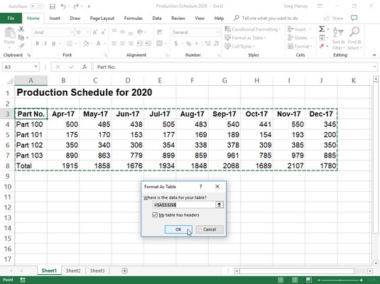Selecting a format from the Table Styles gallery and indicating its range in the Format As Table dialog box.

This dialog box contains a Where Is the Data for Your Table text box that shows the address of the cell range currently selected by the marquee and a My Table Has Headers check box.

If Excel does not correctly guess the range of the data table you want to format in Excel 2019, drag through the cell range to adjust the marquee and the range address in the Where Is the Data for Your Table text box. If your data table doesn’t use column headers or, if the table has them, but you still don’t want Excel to add Filter drop-down buttons to each column heading, deselect the My Table Has Headers check box before you click the OK button.

The table formats in the Table Styles gallery are not available if you select multiple nonadjacent cells before you click the Format as Table command button on the Home tab.

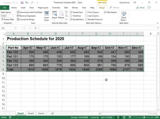After you select a format from the Table Styles gallery, the Design tab appears under the Table Tools contextual tab.

The Design tab enables you to use Live Preview to see how your table would appear. Simply click the Table Styles continuation button on the Design tab of the Ribbon (or Quick Styles button, if it’s displayed) and then position the mouse pointer over any of the format thumbnails in the Table Styles drop-down palette to see the data in your table appear in that table format. Click the button with the triangle pointing downward to scroll up new rows of table formats in the Table Styles group; click the button with the triangle pointing upward to scroll down rows without opening the Table Styles gallery and possibly obscuring the actual data table in the Worksheet area. Click the More button (the one with the horizontal bar above the downward-pointing triangle) to redisplay the Table gallery and then mouse over the thumbnails in the Light, Medium, and Dark sections to have Live Preview apply them to the table.

You can also use the Excel 2019 Tables option on the Quick Analysis tool to format your worksheet data as a table. Simply select the table data (including headings) as a cell range in the worksheet and then click the Tables option on the Quick Analysis tool, followed by the Table option below at the very beginning of the Tables options. Excel then assigns the Table Style Medium 9 style to your table while at same time selecting the Design tab on the Ribbon. Then if you’re not too keen on this table style, you can use Live Preview in the Tables Styles gallery on this tab to find the table formatting that you do want to use.

Customizing table formats in Excel 2019

• Header Row to display the top row with the labels that identify the type of data in each column as well as the Filter buttons for sorting and filtering data in the first row of the table. (This check box is selected by default.)
• Total Row to have Excel add a Total Row to the bottom of the table that displays the sums of each column that contains values. To apply another Statistical function to the values in a particular column, click the cell in that column’s Total Row to display a drop-down list button and then select the function — Average, Count, Count Numbers, Max, Min, Sum, StdDev (Standard Deviation), or Var (Variance).
• Banded Rows to have Excel apply shading to every other row in the table.
• First Column to have Excel display the row headings in the first column of the table in bold.
• Last Column to have Excel display the row headings in the last column of the table in bold.
• Banded Columns to have Excel apply shading to every other column in the table.
• Filter Button to have Excel display drop-down buttons to the right of the entries when the table’s Header Row is displayed that you can use to sort and filter the data in that column. (This check box is selected by default.)

Creating a new custom Table Style in Excel 2019

To create a custom Table Style in Excel 2019, you follow these steps:

1. Format the data in your worksheet as a table using one of the existing styles.
2. On the Design contextual tab of the Tables Tool tab, click the Table Styles More drop-down button and then select the New Table Style option near the bottom of the gallery.

   The New Table Style dialog box appears.

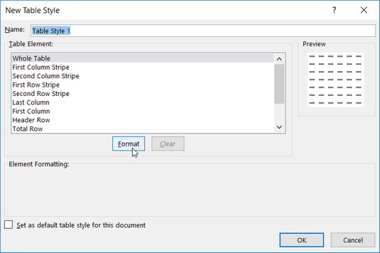   Use the options in the New Table Style dialog box to create a new custom table style to add to the Table Styles gallery.
3. Replace the generic, table style name, Table Style 1, with a more descriptive name in the Name text box.
4. Modify each of the individual table components in the Table Elements list box (from Whole Table through Last Total Cell) with the custom formatting you want included in your new custom table style.

   To customize the formatting for a table element, select its name in the Table Element list box. After you select the element, click the Format button to open the Format Cells dialog box where you can change that element’s font style and/or color on its Font tab, the border style and/or color on its Border tab, or the fill effect and/or color on its Fill tab.

   Note that when customizing a First or Second Column or Row Stripe element (that controls the shading or banding of table’s column or row), in addition to changing the fill for the banding on the Fill tab of the Format Cells dialog box, you can also increase how many columns or rows are banded by increasing the number in the Stripe Size drop-down list that appears when you select one of the Stripe elements.

   As you assign new formatting to a particular table element, Excel displays a description of the formatting change below the Element Formatting heading of New Table Style dialog box, as long as that table element remains selected in the Table Element list box. When you add a new fill color to a particular element, this color appears in the Preview area of this dialog box regardless of which component is selected in the Table Element list box.

5. (Optional) If you want your new custom table style to become the default table style for all the data tables you format in your workbook, select the Set as Default Table Style for This Document check box.
6. Click the OK button to save the settings for your new custom table style and close the New Table Style dialog box.

If you made changes to the fill formatting for the First or Second Column Stripe element in the custom table style, don’t forget to select the Banded Rows check box in Table Styles Options section on the Table Tools Design tab to make it appear in the formatted data table. So, too, if you made changes to the First or Second Row Stripe, you need to select the Banded Rows check box to make these formats appear.