
You may be asked to compare two lists and pick out the values that are in one list but not the other, or you may need to compare two lists and pick out only the values that exist in both lists. Conditional formatting is an ideal way to accomplish either task.
Highlight values that exist in List1 but not List2
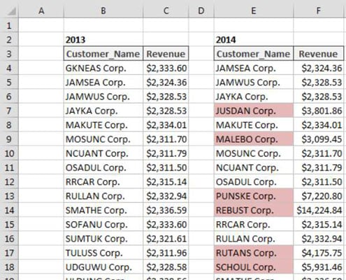
The figure illustrates a conditional formatting exercise that compares customers from 2013 and 2014, highlighting those customers in 2014 who are new customers (they were not customers in 2013).
To build this basic formatting rule, follow these steps:
Select the data cells in your target range (cells E4:E28 in this example), click the Home tab of the Excel Ribbon, and then select Conditional Formatting→New Rule.
This opens the New Formatting Rule dialog box.
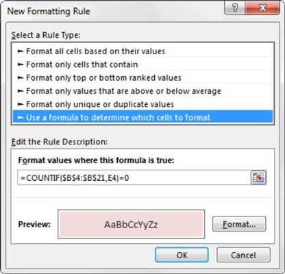
In the list box at the top of the dialog box, click the Use a Formula to Determine which Cells to Format option.
This selection evaluates values based on a formula you specify. If a particular value evaluates to TRUE, the conditional formatting is applied to that cell.
In the formula input box, enter the formula shown with this step.
Note that you use the COUNTIF function to evaluate whether the value in the target cell (E4) is found in your comparison range ($B$4:$B$21). If the value is not found, the COUNTIF function will return a 0, thus triggering the conditional formatting. As with standard formulas, you need to ensure that you use absolute references so that each value in your range is compared to the appropriate comparison cell.
=COUNTIF($B$4:$B$21,E4)=0
Note that in the formula, you exclude the absolute reference dollar symbols ($) for the target cell (E4). If you click cell E4 instead of typing the cell reference, Excel automatically makes your cell reference absolute. It’s important that you don’t include the absolute reference dollar symbols in your target cell because you need Excel to apply this formatting rule based on each cell’s own value.
Click the Format button.
This opens the Format Cells dialog box, where you have a full set of options for formatting the font, border, and fill for your target cell. After you have completed choosing your formatting options, click the OK button to confirm your changes and return to the New Formatting Rule dialog box.
In the New Formatting Rule dialog box, click the OK button to confirm your formatting rule.
If you need to edit your conditional formatting rule, simply place your cursor in any of the data cells within your formatted range and then go to the Home tab and select Conditional Formatting→Manage Rules. This opens the Conditional Formatting Rules Manager dialog box. Click the rule you want to edit and then click the Edit Rule button.
Highlight values that exist in List1 and List2
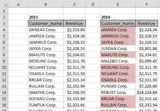
The figure illustrates a conditional formatting exercise that compares customers from 2013 and 2014, highlighting those customers in 2014 who are in both lists.
To build this basic formatting rule, follow these steps:
Select the data cells in your target range (cells E4:E28 in this example), click the Home tab of the Excel Ribbon, and select Conditional Formatting→New Rule.
This opens the New Formatting Rule dialog box.

In the list box at the top of the dialog box, click the Use a Formula to Determine which Cells to Format option.
This selection evaluates values based on a formula you specify. If a particular value evaluates to TRUE, the conditional formatting is applied to that cell.
In the formula input box, enter the formula shown with this step.
Note that you use the COUNTIF function to evaluate whether the value in the target cell (E4) is found in your comparison range ($B$4:$B$21). If the value is found, the COUNTIF function returns a number greater than 0, thus triggering the conditional formatting. As with standard formulas, you need to ensure that you use absolute references so that each value in your range is compared to the appropriate comparison cell.
=COUNTIF($B$4:$B$21,E4)>0
Note that in the formula, you exclude the absolute reference dollar symbols ($) for the target cell (E4). If you click cell E4 instead of typing the cell reference, Excel automatically makes your cell reference absolute. It’s important that you don’t include the absolute reference dollar symbols in your target cell because you need Excel to apply this formatting rule based on each cell’s own value.
Click the Format button.
This opens the Format Cells dialog box, where you have a full set of options for formatting the font, border, and fill for your target cell. After you have completed choosing your formatting options, click the OK button to confirm your changes and return to the New Formatting dialog Rule box.
Back in the New Formatting Rule dialog box, click the OK button to confirm your formatting rule.
If you need to edit your conditional formatting rule, simply place your cursor in any of the data cells within your formatted range and then go to the Home tab and select Conditional Formatting→Manage Rules. This opens the Conditional Formatting Rules Manager dialog box. Click the rule you want to edit and then click the Edit Rule button.