For certain values of input (usually denoted by the letters x or n), you have a corresponding answer using the math that defines the function. For instance, a function like f(n) = 2n tells you that when your input is a number n, your answer is the number n multiplied by 2.
Using the size of the input does make sense given that this is a time-critical age and people's lives are crammed with a growing quantity of data. Making everything a mathematical function is a little less intuitive, but a function describing how an algorithm relates its solution to the quantity of data it receives is something you can analyze without specific hardware or software support. It's also easy to compare with other solutions, given the size of your problem. Analysis of algorithms is really a mind-blowing concept because it reduces a complex series of steps into a mathematical formula.
Moreover, most of the time, an analysis of algorithms isn't even interested in defining the function exactly. What you really want to do is compare a target function with another function. These comparison functions appear within a set of proposed functions that perform poorly when contrasted to the target algorithm. In this way, you don't have to plug numbers into functions of greater or lesser complexity; instead, you deal with simple, premade, and well-known functions. It may sound rough, but it's more effective and is similar to classifying the performance of algorithms into categories, rather than obtaining an exact performance measurement.
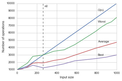
The set of generalized functions is called Big O notation, and you often encounter this small set of functions (put into parentheses and preceded by a capital O) used to represent the performance of algorithms. The figure shows the analysis of an algorithm. A Cartesian coordinate system can represent its function as measured by RAM simulation, where the abscissa (the x coordinate) is the size of the input and the ordinate (the y coordinate) is its resulting number of operations.
You can see three curves represented. Input size matters. However, quality also matters (for instance, when ordering problems, it's faster to order an input which is already almost ordered). Consequently, the analysis shows a worst case, f1(n), an average case, f2(n), and a best case, f3(n).
Even though the average case might give you a general idea, what you really care about is the worst case, because problems may arise when your algorithm struggles to reach a solution. The Big O function is the one that, after a certain n0 value (the threshold for considering an input big), always results in a larger number of operations given the same input than the worst-case function f1. Thus, the Big O function is even more pessimistic than the one representing your algorithm, so that no matter the quality of input, you can be sure that things cannot get worse than that.
Many possible functions can result in worse results, but the choice of functions offered by the Big O notation that you can use is restricted because its purpose is to simplify complexity measurement by proposing a standard. Consequently, this section contains just the few functions that are part of the Big O notation. The following list describes them in growing order of complexity:
- Constant complexity O(1): The same time, no matter how much input you provide. In the end, it is a constant number of operations, no matter how long the input data is. This level of complexity is quite rare in practice.
- Logarithmic complexity O(log n): The number of operations grows at a slower rate than the input, making the algorithm less efficient with small inputs and more efficient with larger ones. A typical algorithm of this class is the binary search.
- Linear complexity O(n): Operations grow with the input in a 1:1 ratio. A typical algorithm is iteration, which is when you scan input once and apply an operation to each element of it.
- Linearithmic complexity O(n log n): Complexity is a mix between logarithmic and linear complexity. It is typical of some smart algorithms used to order data, such as Mergesort, Heapsort, and Quicksort.
- Quadratic complexity O(n2): Operations grow as a square of the number of inputs. When you have one iteration inside another iteration (nested iterations, in computer science), you have quadratic complexity. For instance, you have a list of names and, in order to find the most similar ones, you compare each name against all the other names. Some less efficient ordering algorithms present such complexity: bubble sort, selection sort, and insertion sort. This level of complexity means that your algorithms may run for hours or even days before reaching a solution.
- Cubic complexity O(n3): Operations grow even faster than quadratic complexity because now you have multiple nested iterations. When an algorithm has this order of complexity and you need to process a modest amount of data (100,000 elements), your algorithm may run for years. When you have a number of operations that is a power of the input, it is common to refer to the algorithm as running in polynomial time.
- Exponential complexity O(2n): The algorithm takes twice the number of previous operations for every new element added. When an algorithm has this complexity, even small problems may take forever. Many algorithms doing exhaustive searches have exponential complexity. However, the classic example for this level of complexity is the calculation of Fibonacci numbers.
- Factorial complexity O(n!): A real nightmare of complexity because of the large number of possible combinations between the elements. Just imagine: If your input is 100 objects and an operation on your computer takes 10-6 seconds (a reasonable speed for every computer, nowadays), you will need about 10140 years to complete the task successfully (an impossible amount of time since the age of the universe is estimated as being 1014 years). A famous factorial complexity problem is the traveling salesman problem, in which a salesman has to find the shortest route for visiting many cities and coming back to the starting city.