Keeping Solutions Balanced for Machine Learning

Because data is what dictates the most suitable solution for the prediction problem, you have neither a panacea nor an easy recurrent solution for solving all your machine learning dilemmas.

A commonly referred theorem in the mathematical folklore is the no-free-lunch theorem by David Wolpert and William Macready, which states that “any two optimization algorithms are equivalent when their performance is averaged across all possible problems.” If the algorithms are equivalent in the abstract, no one is superior to the other unless proved in a specific, practical problem. (See this discussion for more details about no-free-lunch theorems; two of them are actually used for machine learning.)

Besides being led into machine learning experimentation by the try-everything principle of the no-free-lunch theorem, you have another rule of thumb to consider: Occam’s razor, which is attributed to William of Occam, a scholastic philosopher and theologian who lived in the fourteenth century.

The Occam’s razor principle states that theories should be cut down to the minimum in order to plausibly represent the truth (hence the razor). The principle doesn’t state that simpler solutions are better, but that, between a simple solution and a more complex solution offering the same result, the simpler solution is always preferred. The principle is at the very foundations of our modern scientific methodology, and even Albert Einstein seems to have often referred to it, stating that “everything should be as simple as it can be, but not simpler.” Summarizing the evidence so far:

• To get the best machine learning solution, try everything you can on your data and represent your data’s performance with learning curves.
• Start with simpler models, such as linear models, and always prefer a simpler solution when it performs nearly as well as a complex solution. You benefit from the choice when working on out-of-sample data from the real world.
• Always check the performance of your solution using out-of-sample examples.

Depicting learning curves

If the chart depicts performance with respect to the quantity of data, it’s a learning curve chart. When it depicts performance with respect to different hyper-parameters or a set of learned features picked by the model, it’s a validation curve chart instead. To create a learning curve chart, you must do the following:

• Divide your data into in-sample and out-of-sample sets (a train/test split of 70/30 works fine, or you can use cross-validation).
• Create portions of your training data of growing size. Depending on the size of the data that you have available for training, you can use 10 percent portions or, if you have a lot of data, grow the number of examples on a power scale such as 10³, 10⁴, 10⁵ and so on.
• Train models on the different subsets of the data. Test and record their performance on the same training data and on the out-of-sample set.
• Plot the recorded results on two curves, one for the in-sample results and the other for the out-of-sample results. If instead of a train/test split you used cross-validation, you can also draw boundaries expressing the stability of the result across multiple validations (confidence intervals) based on the standard deviation of the results themselves.

Examples of learning curves affected by bias (left) and variance (right).

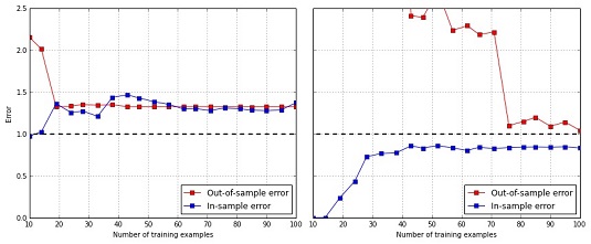
Ideally, you should obtain two curves with different starting error points: higher for the out-of-sample; lower for the in-sample. As the size of the training set increases, the difference in space between the two should reduce until, at a certain number of observations, they become close to a common error value.

Noticeably, after you print your chart, problems arise when

• The two curves tend to converge, but you can’t see on the chart that they get near each other because you have too few examples. This situation gives you a strong hint to increase the size of your dataset if you want to successfully learn with the tested machine learning algorithm.
• The final convergence point between the two curves has a high error, so consequently your algorithm has too much bias. Adding more examples here does not help because you have a convergence with the amount of data you have. You should increase the number of features or use a more complex learning algorithm as a solution.
• The two curves do not tend to converge because the out-of-sample curve starts to behave erratically. Such a situation is clearly a sign of high variance of the estimates, which you can reduce by increasing the number of examples (at a certain number, the out-of-sample error will start to decrease again), reducing the number of features, or, sometimes, just fixing some key parameters of the learning algorithm.