
Overview
An ML neural network consists of simulated neurons, often called units, or nodes, that work with data. Like the neurons in the nervous system, each unit receives input, performs some computation, and passes its result as a message to the next unit. At the output end, the network makes a decision based on its inputs.Imagine a neural network that uses physical measurements of flowers, like irises, to identify the flower’s species. The network takes data like the petal length and petal width of an iris and learns to classify an iris as either setosa, versicolor, or virginica. In effect, the network learns the relationship between the inputs (the petal variables) and the outputs (the species).
The image below shows an artificial neural network that classifies irises. It consists of an input layer, a hidden layer, and an output layer. Each unit connects with every unit in the next layer. Numerical values called weights are on each connection. Weights can be positive or negative. To keep the image from getting cluttered, you only see the weights on the connections from the input layer to the hidden layer.
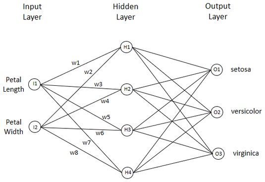 An artificial neural network that learns to classify irises.
Input layer and hidden layer
The data points are represented in the input layer. This one has one input unit (I1) that holds the value of petal length and another (I2) that holds the value of petal width. The input units send messages to another layer of four units, called a hidden layer. The number of units in the hidden layer is arbitrary, and picking that number is part of the art of neural network creation.Each message to a hidden layer unit is the product of a data point and a connection weight. For example, H1 receives I1 multiplied by w1 along with I2 multiplied by w2. H1 processes what it receives.
What does “processes what it receives” mean? H1 adds the product of I1 and w1 to the product of I2 and w2. H1 then has to send a message to O1, O2, and O3.
What is the message it sends? It’s a number in a restricted range, produced by H1’s activation function. Three activation functions are common. They have exotic, math-y names: hyperbolic tangent, sigmoid, and rectified linear unit.
Without going into the math, I’ll just tell you what they do. The hyperbolic tangent (known as tanh) takes a number and turns it into a number between –1 and 1. Sigmoid turns its input into a number between 0 and 1. Rectified linear unit (ReLU) replaces negative values with 0.
By restricting the range of the output, activation functions set up a nonlinear relationship between the inputs and the outputs. Why is this important? In most real-world situations, you don’t find a nice, neat linear relationship between what you try to predict (the output) and the data you use to predict it (the inputs).
One more item gets added into the activation function. It’s called bias. Bias is a constant that the network adds to each number coming out of the units in a layer. The best way to think about bias is that it improves the network’s accuracy.
Bias is much like the intercept in a linear regression equation. Without the intercept, a regression line would pass through (0,0) and might miss many of the points it’s supposed to fit.
To summarize: A hidden unit like H1 takes the data sent to it by I1 (Petal length) and I2 (Petal width), multiplies each one by the weight on its interconnection (I1 × w1 and I2 × w2), adds the products, adds the bias, and applies its activation function. Then it sends the result to all units in the output layer.Output layer
The output layer consists of one unit (O1) for setosa, another (O2) for virginica, and another (O3) for versicolor. Based on the messages they receive from the hidden layer, the output units do their computations just as the hidden units do theirs. Their results determine the network’s decision about the species for the iris with the given petal length and petal width. The flow from input layer to hidden layer to output layer is called feedforward.How it all works
Where do the interunit connection weights come from? They start out as numbers randomly assigned to the interunit connections. The network trains on a data set of petal lengths, petal widths, and the associated species. On each trial, the network receives a petal length and a petal width and makes a decision, which it then compares with the correct answer. Because the initial weights are random, the initial decisions are guesses.Each time the network’s decision is incorrect, the weights change based on how wrong the decision was (on the amount of error, in other words). The adjustment (which also includes changing the bias for each unit) constitutes “learning." One way of proceeding is to adjust the weights from the output layer back to the hidden layer and then from the hidden layer back to the input layer. This is called backpropagation because the amount of error “backpropagates” through the layers.
A network trains until it reaches a certain level of accuracy or a preset number of iterations through the training set. In the evaluation phase, the trained network tackles a new set of data.
This three-layer structure is just one way of building a neural network. Other types of networks are possible.