
You may find it easier to customize and work with your pivot table in Excel 2013 if you move the chart to its own chart sheet in the workbook, even though Excel automatically creates all new pivot charts on the same worksheet as the pivot table. To move a new pivot chart to its own chart sheet in the workbook, you follow these steps:
Click the Analyze tab under the PivotChart Tools contextual tab to bring its tools to the Ribbon.
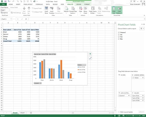
If the PivotChart Tools contextual tab doesn’t appear at the end of your Ribbon, click anywhere on the new pivot chart to make this tab reappear.
Click the Move Chart button in the Actions group.
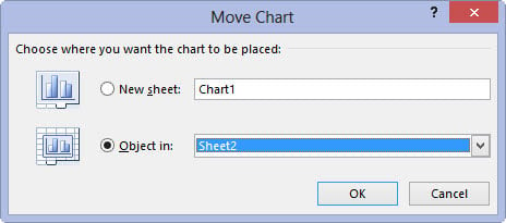
Excel opens a Move Chart dialog box.
Click the New Sheet button in the Move Chart dialog box.
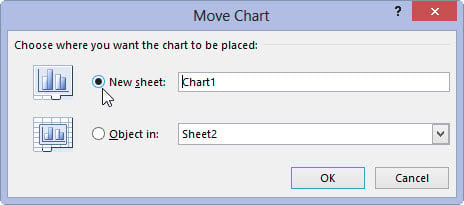
Excel will open a New Sheet.
Rename the generic Chart1 sheet name in the accompanying text box by entering a more descriptive name there.
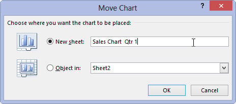
This is an optional step, but may help you organize later when Excel’s default names are too generic.
Click OK to close the Move Chart dialog box and open the new chart sheet with your pivot chart.
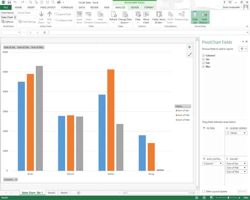
You can see a clustered column pivot chart after moving the chart to its own chart sheet in the workbook.