
The Chart Elements button (with the plus sign icon) that appears when your chart is selected in Excel 2013 contains a list of the major chart elements that you can add to your chart. To add an element to your chart, click the Chart Elements button to display an alphabetical list of all the elements, Axes through Trendline.
To add a particular element missing from the chart, select the element’s check box in the list to put a check mark in it. To remove a particular element currently displayed in the chart, select the element’s check box to remove its check mark.
To add or remove just part of a particular chart element or, in some cases as with the Chart Title, Data Labels, Data Table, Error Bars, Legend, and Trendline, to also specify its layout, you select the desired option on the element’s continuation menu.
So, for example, to reposition a chart’s title, you click the continuation button attached to Chart Title on the Chart Elements menu to display and select from among the following options on its continuation menu:
Above Chart to add or reposition the chart title so that it appears centered above the plot area
Centered Overlay Title to add or reposition the chart title so that it appears centered at the top of the plot area
More Options to open the Format Chart Title task pane on the right side of the Excel window where you can use the options when you select the Fill & Line, Effects, and Size and Properties buttons under Title Options and the Text Fill & Outline, Text Effects, and the Textbox buttons under Text Options in this task pane to modify almost any aspect of the title’s formatting
How to add data labels in Excel 2013
Data labels identify the data points in your chart by displaying values from the cells of the worksheet represented next to them. To add data labels to your selected chart and position them, click the Chart Elements button next to the chart and then select the Data Labels check box before you select one of the following options on its continuation menu:
Center to position the data labels in the middle of each data point
Inside End to position the data labels inside each data point near the end
Inside Base to position the data labels at the base of each data point
Outside End to position the data labels outside of the end of each data point
Data Callout to add text labels and values that appear within text boxes that point to each data point
More Options to open the Format Data Labels task pane where you can use the options that appear when you select the Fill & Line, Effects, Size & Properties, and Label Options buttons under Label Options and the Text Fill & Outline, Text Effects, and Textbox buttons under Text Options in the task pane to customize any aspect of the appearance and position of the data labels.
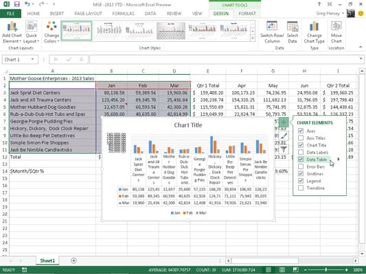
How to add data tables in Excel 2013
Sometimes, instead of data labels that can easily obscure the data points in the chart, you’ll want Excel to draw a data table beneath the chart showing the worksheet data it represents in graphic form.
To add a data table to your selected chart and position and format it, click the Chart Elements button next to the chart and then select the Data Table check box before you select one of the following options on its continuation menu:
With Legend Keys to have Excel draw the table at the bottom of the chart, including the color keys used in the legend to differentiate the data series in the first column
No Legend Keys to have Excel draw the table at the bottom of the chart without any legend
More Options to open the Format Data Table task pane on the right side where you can use the options that appear when you select the Fill & Line, Effects, Size & Properties, and Table Options buttons under Table Options and the Text Fill & Outline, Text Effects, and Textbox buttons under Text Options in the task pane to customize almost any aspect of the data table
This data table includes the legend keys as its first column.
If you decide that displaying the worksheet data in a table at the bottom of the chart is no longer necessary, simply click the None option on the Data Table button’s drop-down menu on the Layout tab of the Chart Tools contextual tab.