The graphs of the inverse trig functions are relatively unique; for example, inverse sine and inverse cosine are rather abrupt and disjointed. These graphs are important because of their visual impact. Especially in the world of trigonometry functions, remembering the general shape of a function’s graph goes a long way toward helping you remember more about the function values and using those values effectively.
Sine and cosine graphs sort of go together because they have a common characteristic. The input values for both y = sin–1 x and y = cos–1 x are all the numbers from –1 to 1. The inputs are restricted to those values because they’re the output values of the sine and cosine.
But the output, or range, values for these two inverse functions are different. The range of y = sin–1 x consists of angles in the first and fourth quadrants. In radians, the range is
in approximate decimal values, the range is –1.571 to 1.571. The range of y = cos–1 x, on the other hand, consists of angles in the first and second quadrants, or angles from 0 to π. In approximate decimal values, that range is 0 to 3.142.
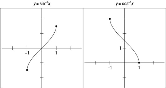
The figure shows what the graphs of inverse sine and cosine look like.
The points indicated on the graphs are at x = –1 and x = 1. These points are the extreme values of the inputs. The y-values of the graph represent the angle measures. If you want to find a point on either graph, just find some number between –1 and 1, and find the place on the graph corresponding to that x-value.