This case study begins with model construction, starting from basic physics. Special consideration is given to incorporate wind resistance and include as a system disturbance, the onset of a hill. The laws of motion say that given a vehicle mass m and engine supplied force cw(t), where c is proportionality constant and 0 ≤ w(t) ≤ 1 represents the engine throttle, Ftot(t) = mv(t) = cw(t), t ≥ 0.
![[Credit: Illustration by Mark Wickert, PhD]](https://www.dummies.com/wp-content/uploads/378980.image0.jpg)
Air resistance, proportional to the velocity squared times constant ρ, produces drag on the vehicle. Additionally when the vehicle encounters a hill (the system disturbance described in the introduction) of angle θ, gravity creates a second counter force, mg sin(θ), where g is the gravitational constant of 9.8 m/s2. A small angle is assumed in this case, so the following is valid.
The equation of motion is now
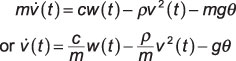
where the last line is divided through by the mass m. This is a nonlinear differential equation in terms of the vehicle velocity v(t) because of the appearance of v2(t), the air resistance term.
Observe the nonlinear differential equation
Although the nonlinear differential equation is not in a form suitable for design of a cruise control, there are some interesting observations that can be made. This understanding also helps with the linearizing process.
When the vehicle is on the flat (θ = 0) and at the maximum throttle value of 1.0, the nonlinear differential equation reduces to
The maximum velocity will be reached as t becomes large. At maximum velocity the acceleration must be zero, so
The equation further simplifies to
Don’t try this at home with your car!
A second observation is that the vehicle stalls when climbing a hill at full throttle for some critical angle θs. You first need to know that stall means the vehicle velocity is zero and the acceleration is zero. From the full nonlinear differential equation
You now solve for θs as sin–1[c/(mg)]. Note this analysis assumes that the vehicle stays in a fixed gear. In driving your own car you probably downshift to the lowest gear to avoid stalling.
The third observation is the solution to the nonlinear differential equation at maximum throttle and θ = 0. Begin by defining the constant
the differential equation with this T inserted becomes:
The exact solution to this simplified form is v(t) = vmaxtanh(t / T). You can verify this is a valid solution by inserting it back into the differential equation and see that the equation is satisfied. This solution gives you the velocity profile versus time with the accelerator held to the floor.
Note this doesn’t quite apply to a real car because the model does not take into account gear shifting with a transmission. By plotting v(t) for a given vmax and T you can see approximately how long it takes to accelerate to a particular cruising velocity, for example, 0 to 60 mph in 10 seconds.
Linearize to a nominal cruising velocity
To linearize the differential equation for a nominal cruise velocity of v0 < vmax and corresponding throttle setting of 0 < w0 < 1, use a one-term Taylor series expansion. In calculus, you learn that any function, say y = f(x), can be approximated near the point x0 using f(x0) and its derivatives evaluated at x0. A one term approximation is linear in x – x0, that is
If f(x) = x2 the expansion becomes
because f '(x) = 2x evaluated at x0 is 2x0.
For the problem at hand, you want to expand with respect to the nominal velocity v0 and throttle setting w0. Make substitutions into the original differential equation as follows:
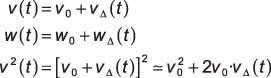
represent the deviation of velocity and throttle settings away from the nominal values. These are the new modeling parameters. In the original differential equation:
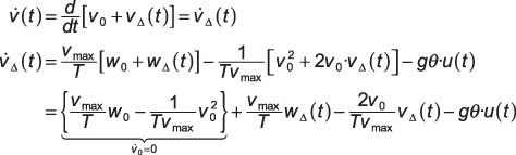
where a step function is included on the hill gravity term to model the hill onset to t = 0. Note in the last line
is zero because this is the nominal constant operating point, which also corresponds to the throttle setting w0. If you define the time constant
the now linearized differential equation becomes