Simulate the Time Domain for the CD/DVD Case Study with PyLab

You can simulate the complete CD/DVD drive control system by using a step function input for r(t), which is the commanding signal for the sled positioner. The output should be scaled in millimeters for a voltage signal at the input. The convolution theorem states that y(t) = r(t) x h(t); h(t) is the impulse response of the closed-loop system function H(s).

To numerically crank out the time-domain system output y(t) for arbitrary input r(t), you can use the SciPy signal package function ty,y,x_state = lsim((b,a),r,t). The function numerically solves the linear constant coefficient differential equation, given the numerator and denominator polynomials corresponding to H(s) = B(s)/A(s) are stored in the ndarrays b and a, respectively.

The input r is a sampled version of r(t) that corresponds to the time index array t. Choose the time spacing carefully to ensure adequate samples are taken of small time constant poles and zeros.

In [<b>103</b>]: b,a = ssd.position_CD(50,'fb_approx')
In [<b>104</b>]: ty,y,x_state = signal.lsim((b,a),10.0*ones(len(t)),t)
In [<b>105</b>]: plot(ty,y)
In [<b>106</b>]: # repeat for Ka = 25,75,& 100 (4 plots total)

The input is a step of amplitude 10, meaning that you command the sled positioner to move 10 mm from its zero reference position. The results are shown here.

Credit: Illustration by Mark Wickert, PhD

As expected, when the command input steps to 10, the sled position moves to 10 mm. The exact and simplified model results overlay each other when K_a = 100. In all cases, the sled doesn’t move instantly. Are you disappointed?

The motor has a limited amount of torque, and it must overcome the inertia of the mechanical load, which takes time. Increasing the amplifier gain does make the position change faster, but it also introduces more overshoot in the response. This matters because you can’t read/write data while the sled position is settling to a new position value. Fortunately, this position change is needed only when changing tracks.

As a final bit of analysis, check to see whether the steady-state value of y(t) does indeed settle to 10 mm. The final value theorem states that

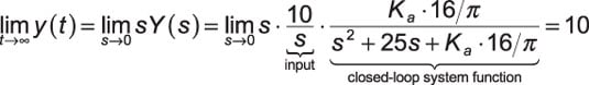
The system is stable, and by analysis, you now know that the final value of the output is the desired value — no errors.