How to Work and Verify Convolution Integral and Sum Problems

Mastering convolution integrals and sums comes through practice. Here are detailed analytical solutions to one convolution integral and two convolution sum problems, each followed by detailed numerical verifications, using PyLab from the IPython interactive shell (the QT version in particular).

Continuous-time convolution

Here is a convolution integral example employing semi-infinite extent signals. Consider the convolution of x(t) = u(t) (a unit step function) and

(a real exponential decay starting from t = 0). The figure provides a plot of the waveforms.

Credit: Illustration by Mark Wickert, PhD

The output support interval is

You need two cases (steps) to form the analytical solution valid over the entire time axis.

• Case 1: Using Figure b, you can clearly see that for t < 0, it follows that y(t) = 0.

• Case 2: Again looking at Figure b, you see that for t ≥ 0, some overlap always occurs between the two signals of the integrand. The convolution integral output is

  

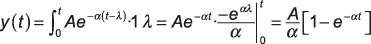
Putting the two pieces together, the analytical solution for y(t) is

To verify this analytical solution, follow the same steps you used in the earlier example:

1. Write a simple Python function for plotting the analytical solution:

   In [<b>133</b>]: def expo_conv(t,A,alpha):
        ...: y = zeros(len(t))
        ...: for k, tk in enumerate(t):
        ...:     if tk >= 0:
        ...:         y[k] = A/alpha*(1 - exp(-alpha*tk))
        ...: return y

2. For the numerical convolution, use ssd.conv_integral(). You first write Python code in the command window to generate the signals x(t) and h(t) and then carry out the convolution:

   In [<b>135</b>]: t = arange(-4,14,.01)
   In [<b>136</b>]: xc2 = ssd.step(t)
   In [<b>137</b>]: hc2 = ssd.step(t)*exp(-1*t)
   In [<b>138</b>]: yc2_num,tyc2 = ssd.conv_integral(xc2,t,hc2,t,('r','r'))
   Output support: (-8.00, +5.99)
   In [<b>143</b>]: subplot(211)
   In [<b>144</b>]: plot(t,expo_conv(t,1,1))
   In [<b>149</b>]: subplot(212)
   In [<b>151</b>]: plot(tyc2,yc2_num)
   In [<b>156</b>]: savefig('c2_outputs.pdf')

   Notice that the fifth argument of the conv_integral function is (‘r’,’r’). For signals with infinite extent to the right, each ‘r’ tells the function that both signals are right-sided and to return only the valid support interval under this assumption.

   The default values of (‘f’,’f’) means finite support for both signals over the input time axes t1 and t2 given to the function.

   

   Credit: Illustration by Mark Wickert, PhD

Once again, the agreement is excellent, so the analytical solution is verified.

Verify discrete-time convolution

For the case of discrete-time convolution, here are two convolution sum examples. The first employs finite extent sequences (signals) and the second employs semi-infinite extent signals. You encounter both types of sequences in problem solving, but finite extent sequences are the usual starting point when you’re first working with the convolution sum.

Two finite length sequences

Consider the convolution sum of the two sequences x[n] and h[n], shown here, along with the convolution sum setup.

Credit: Illustration by Mark Wickert, PhD

When convolving finite duration sequences, you can do the analytical solution almost by inspection or perhaps by using a table (even a spreadsheet) to organize the sequence values for each value of n, which produces a nonzero overlap between h[k] and x[n – k].

The support interval for the output follows the rule given for the continuous-time domain. The output y[n] starts at the sum of the two input sequence starting points and ends at the sum of input sequence ending points. For the problem at hand this corresponds to y[n] starting at [0 + –1] = –1 and ending at [3 + 1] = 4.

Looking at Figure b, you can see that as n increases from n < –1, first overlap occurs when n = –1. The last point of overlap occurs when n – 3 = 1 or n = 4. You can set up a spreadsheet table to evaluate the six sum-of-products related to the output support interval.

Credit: Illustration by Mark Wickert, PhD

To verify these hand (spreadsheet) calculation values, use Python functions in ssd.py to perform the convolution sum. The convolution sum function is y, ny = ssd.conv_sum(x1, nx1, x2, nx2, extent=('f', 'f')).

In [<b>208</b>]: n = arange(-4,6)
In [<b>209</b>]: xd1 = 2*ssd.drect(n,4)
In [<b>210</b>]: hd1 = 1.5*ssd.dimpulse(n) - 0.5*ssd.drect(n+1,3)
In [<b>211</b>]: yd1_num, nd1 = ssd.conv_sum(xd1,n,hd1,n)
Output support: (-8, +10)
In [<b>212</b>]: stem(nd1,yd1_num)

See the numerical results output sequence plotted.

Credit: Illustration by Mark Wickert, PhD

The results of the numerical calculation indeed correspond to the hand calculation.

One finite and one semi-infinite sequence

As a second example of working with the convolution consider a finite duration pulse sequence of 2M + 1 points convolved with the semi-infinite exponential sequence aⁿ u[n] (a real exponential decay starting from n = 0). A plot of the waveforms is given here.

Credit: Illustration by Mark Wickert, PhD

With the help of Figure b, you have three cases to consider in the evaluation of the convolution for all values of n. The support interval for the convolution is

Here are the steps for each case:

• Case 1: From Figure b, you see that for n + M < 0 or n < –M no overlap occurs between the two sequences of the sum, so y[n] = 0.

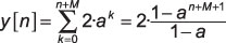
• Case 2: Partial overlap between the two sequences occurs when n + M ≥ 0 and n – M ≤ 0 or –M ≤ n ≤ M. The sum limits start at k = 0 and end at k = n + M. Using the finite geometric series sum formula, the convolution sum evaluates to

  

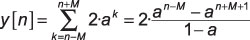
• Case 3: Full overlap occurs when n – M > 0 or n > M. The sum limits under this case run from k = n – M to k = n + M. Again, using the finite geometric series sum formula, the convolution sum evaluates to

  

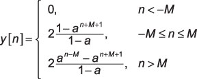
Putting the pieces together, the complete analytical solution for this problem is

To compare the analytical solution with the numerical solution, you follow the steps of plotting the analytical function against a plot of the actual convolution sum:

1. Write a Python function to evaluate y[n] as a piecewise function:

   In [<b>239</b>]: def expo_pulse_conv(n,a,M):
        ...: y = zeros(len(n))
        ...: for k, nk in enumerate(n):
        ...:     if nk >= -M and nk <= M:
        ...:         y[k] = 2*(1 - a**(nk+M+1))/(1 - a)
        ...:     elif nk > M:
        ...:         y[k] = 2*(a**(nk-M) - a**(nk+M+1))/(1 - a)
        ...: return y

2. Find the actual convolution sum by using the function conv_sum() and then plotting the results:

   In [<b>255</b>]: n = arange(-5,30) # n values for x[n] & h[n]
   In [<b>256</b>]: xd2 = 2*ssd.drect(n+4,9) # create x[n]
   In [<b>257</b>]: hd2 = ssd.dstep(n)*0.6**n # create h[n]
   In [<b>258</b>]: yd2_num,nd2 = ssd.conv_sum(xd2,n,hd2,n,('f','r'))
   Output support: (-10, +24)
   In [<b>259</b>]: subplot(211)
   In [<b>260</b>]: stem(n,expo_pulse_conv(n,0.6,4)) # analytical
   In [<b>265</b>]: subplot(212)
   In [<b>266</b>]: stem(nd2,yd2_num) # numerical 
   In [<b>271</b>]: savefig('d2_outputs.pdf')

   Use the fifth argument to the conv_sum() function to declare the extent of the second input sequence to right-sided (‘r’), as opposed to the default value of finite (‘f’). This setting ensures that the function doesn’t return invalid results.

   

   Credit: Illustration by Mark Wickert, PhD

Here, you see that the piecewise analytical solution compares favorably to the direct convolution sum numerical calculation.