To study a range of frequencies, you use Bode plots. Bode plots help you visualize how poles and zeros affect the frequency response of a circuit. You can express the frequency response gain |T(jω)| in terms of decibels. Using decibels compresses the magnitude and the frequency in a logarithmic scale so you don’t need more than 10 feet of paper for your plots. Decibels are defined as |T(jω)|db = 20log10|T(jω)|.
For example, if the gain is |T(jω)|, the gain in decibels is 40 dB. Also, a gain of 1 is 0 dB.
At the cutoff frequency ωC, which is commonly defined as TMAX /√2, you have the following gain:
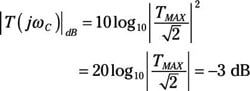
Therefore, the cutoff frequency is also referred to as the –3 dB point or the half-power point.
Why? Because the previous set of equations involving a transfer function can be viewed as the square of either the voltage or the current transfer function. Squaring the transfer function gives you the power ratio between the output and input signal transforms because the square of the voltage or current is proportional to power.
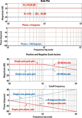
The log-frequency plots of the gain |T(jω)| and phase θ(ω) are called Bode plots, or Bode diagrams.
A basic Bode plot
Bode plots come in pairs to describe the frequency response of circuits. Usually, you have
-
A log-frequency gain plot in decibels given in the top diagram
-
A log-frequency phase plot in degrees given in the bottom diagram
Here is a sample Bode plot.
The horizontal axis usually comes in one of the following log-frequency scales, usually decades:
-
Octaves: An octave has a frequency range whose upper limit is twice the lower limit (2:1 ratio). For example, the voice usually ranges from 2 kHz to 4 kHz, spanning about 1 octave.
-
Decades: A decade has a range with a 10:1 ratio. For example, human hearing usually ranges from 20 Hz to 20 kHz (20 × 103 Hz), so it spans 3 decades.
Poles, zeros, and scale factors: Picturing Bode plots from transfer functions
Most of the time, you use engineering software to draw Bode plots. But you can approximate Bode plots by hand — or at least notice when the computer-generated plot is messed up — if you understand how the transfer function’s poles and zeros shape the frequency response. The poles, of course, are the roots of the transfer function’s denominator, and zeros are the roots of its numerator.
This table shows some basic, approximate rules to bear in mind when examining transfer functions and Bode plots.
| Characteristic of the Transfer Function, T(jù) | Effects on the Gain Plot, |T(jù)|dB | Effects on the Phase Plot, jèdB |
|---|---|---|
| Scale factor (gain) | Shifts the entire gain plot up or down without changing the cutoff (corner) frequencies | The phase Bode plot is un-affected if the scale factor is positive. If the scale factor is negative, the phase Bode plot shifts by ±180°. |
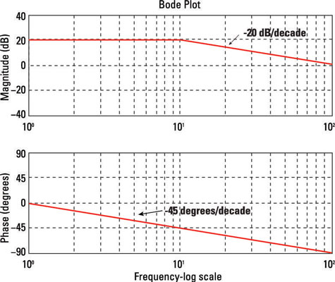
| Real pole | Introduces a slope of –20 dB/decade to the gain Bode plot, starting at the pole frequency | The phase Bode plot rolls off at a slope of –45°/decade. The phase at the pole is –45°. For frequencies greater than 10 times the pole frequency, the phase angle contributed by a single pole is approximately –90°. |
| Real zero | Introduces a slope of +20 dB/decade to the gain Bode plot, starting at the zero frequency | The phase Bode plot rolls off at a slope of +45°/decade. The phase at the zero is +45°. For frequencies greater than 10 times the zero frequency, the phase angle contributed by a single real zero is approximately +90°. |
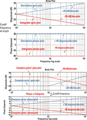
| Integrator | Introduces a real pole at the origin; a real pole at the origin (an integrator 1/s) has a gain slope of –20 dB/decade passing through 0 dB at ω = 1 | The angle contributed by an integrator is –90° at all frequencies. |
| Differentiator | Introduces a real zero at the origin; a zero at the origin (a differentiator) has a gain slope of +20 dB/decade passing through at 0 dB at ù = 1 | The angle contributed by a differentiator is +90° at all frequencies. |
| Complex pair of poles | Provides a slope of –40 dB/decade | The phase Bode plot has a slope of –90°/decade. The phase at the complex pole frequency is –90°. For frequencies greater than 10 times the cutoff frequency, the phase angle contributed by a complex pair of poles is approximately –180°. |
| Complex pair of zeros | Provides a slope of +40 dB/decade | The phase Bode plot has a slope of +90°/decade. The phase at the complex zero frequency is +90°. For frequencies greater than 10 times the cutoff frequency, the phase angle contributed by a complex pair of zeros is approximately +180°. |