With either base R graphics or ggplot 2, the first step is to set up a vector of the values that the density functions will work with:
t.values <- seq(-4,4,.1)
After the graphs are complete, you'll put the infinity symbol on the legends to denote the df for the standard normal distribution. To do that, you have to install a package called grDevices: On the Packages tab, click Install, and then in the Install Packages dialog box, type grDevices and click Install. When grDevices appears on the Packages tab, select its check box.
With grDevices installed, this adds the infinity symbol to a legend:
expression(infinity)
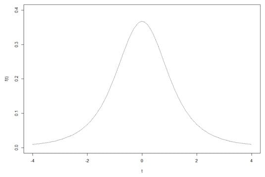
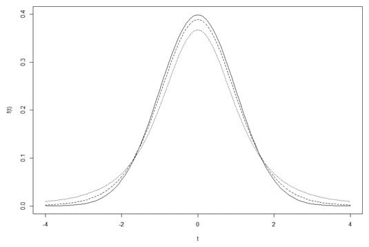
Begin with the plot() function, and plot the t-distribution with 3 df:
plot(x = t.values,y = dt(t.values,3), type = "l", lty = "dotted", ylim = c(0,.4), xlab = "t", ylab = "f(t)")
The first two arguments are pretty self-explanatory. The next two establish the type of plot — type = "l" means line plot (that's a lowercase "L" not the number 1), and lty = "dotted" indicates the type of line. The ylim argument sets the lower and upper limits of the y-axis — ylim = c(0,.4). A little tinkering shows that if you don't do this, subsequent curves get chopped off at the top. The final two arguments label the axes. This figureshows the graph so far:
The next two lines add the t-distribution for df=10, and for the standard normal (df = infinity):
lines(t.values,dt(t.values,10),lty = "dashed")
lines(t.values,dnorm(t.values))
The line for the standard normal is solid (the default value for lty). This figure shows the progress. All that's missing is the legend that explains which curve is which.
One advantage of base R is that positioning and populating the legend is not difficult:
legend("topright", title = "df",legend =
c(expression(infinity),"10","3"), lty =
c("solid","dashed","dotted"), bty = "n")
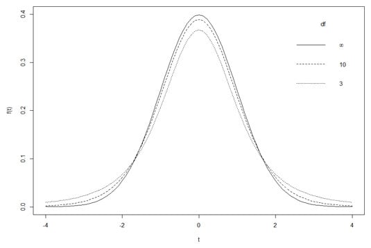
The first argument positions the legend in the upper-right corner. The second gives the legend its title. The third argument is a vector that specifies what's in the legend. As you can see, the first element is the infinity expression, corresponding to the df for the standard normal. The second and third elements are the df for the remaining two t-distributions. You order them this way because that's the order in which the curves appear at their centers. The lty argument is the vector that specifies the order of the linetypes (they correspond with the df). The final argument bty="n" removes the border from the legend.
And this produces the following figure.