
by using a sample mean,
plus or minus a margin of error. The result is called a confidence interval for the population mean,
In many situations, you don’t know
so you estimate it with the sample standard deviation, s. But if the sample size is small (less than 30), and you can’t be sure your data came from a normal distribution. (In the latter case, the Central Limit Theorem can’t be used.) In either situation, you can’t use a z*-value from the standard normal (Z-) distribution as your critical value anymore; you have to use a larger critical value than that, because of not knowing what
is and/or having less data.
The formula for a confidence interval for one population mean in this case is
is the critical t*-value from the t-distribution with n – 1 degrees of freedom (where n is the sample size).
The t-table
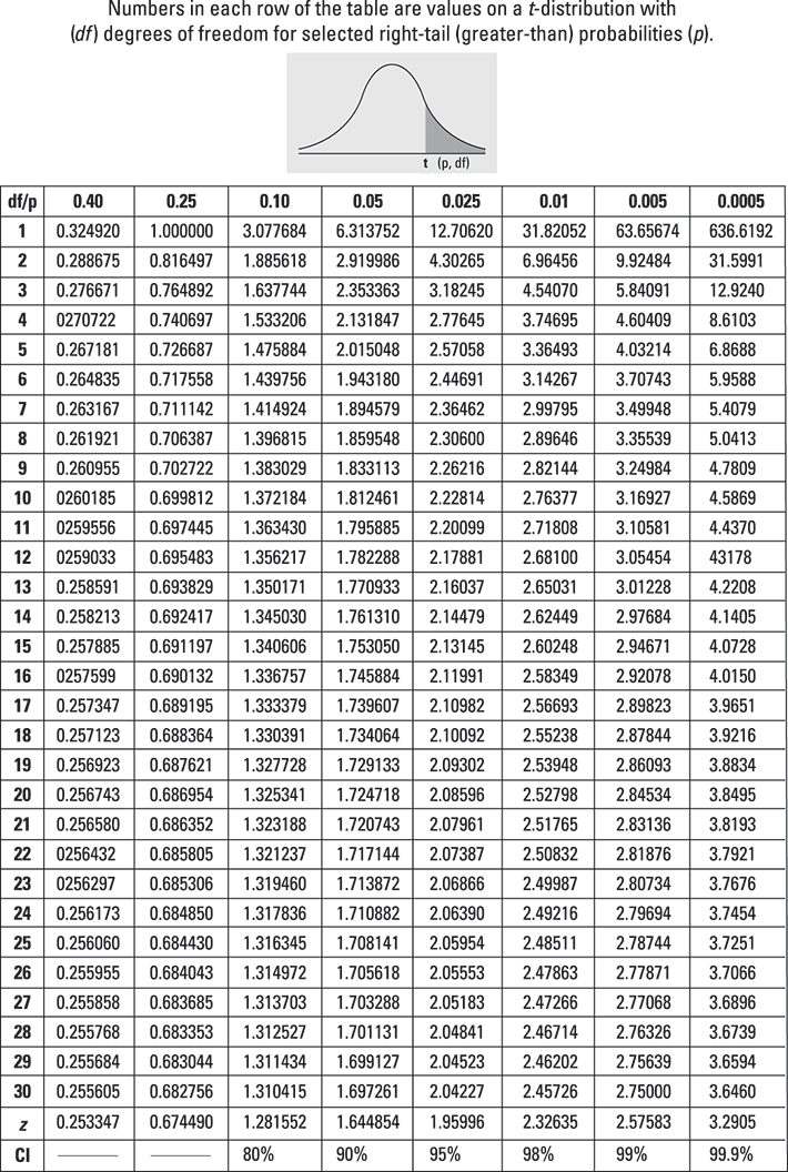
The t*-values for common confidence levels are found using the last row of the t-table above.
The t-distribution has a shape similar to the Z-distribution except it’s flatter and more spread out. For small values of n and a specific confidence level, the critical values on the t-distribution are larger than on the Z-distribution, so when you use the critical values from the t-distribution, the margin of error for your confidence interval will be wider. As the values of n get larger, the t*-values are closer to z*-values.
To calculate a CI for the population mean (average), under these conditions, do the following:-
Determine the confidence level and degrees of freedom and then find the appropriate t*-value.
Refer to the preceding t-table.
-
Find the sample mean

and the sample standard deviation (s) for the sample.
-
Multiply t* times s and divide that by the square root of n.
This calculation gives you the margin of error.
-
Take

plus or minus the margin of error to obtain the CI.
The lower end of the CI is

minus the margin of error, whereas the upper end of the CI is

plus the margin of error.
Here's an example of how this works
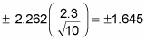
For example, suppose you work for the Department of Natural Resources and you want to estimate, with 95 percent confidence, the mean (average) length of all walleye fingerlings in a fish hatchery pond. You take a random sample of 10 fingerlings and determine that the average length is 7.5 inches and the sample standard deviation is 2.3 inches.-
Because you want a 95 percent confidence interval, you determine your t*-value as follows:
The t*-value comes from a t-distribution with 10 – 1 = 9 degrees of freedom. This t*-value is found by looking at the t-table. Look in the last row where the confidence levels are located, and find the confidence level of 95 percent; this marks the column you need. Then find the row corresponding to df = 9. Intersect the row and column, and you find t* = 2.262. This is the t*-value for a 95 percent confidence interval for the mean with a sample size of 10. (Notice this is larger than the z*-value, which would be 1.96 for the same confidence interval.)
-
You know that the average length is 7.5 inches, the sample standard deviation is 2.3 inches, and the sample size is 10. This means
-
Multiply 2.262 times 2.3 divided by the square root of 10. The margin of error is, therefore,
-
Your 95 percent confidence interval for the mean length of all walleye fingerlings in this fish hatchery pond is

(The lower end of the interval is 7.5 – 1.645 = 5.86 inches; the upper end is 7.5 + 1.645 = 9.15 inches.)
With a smaller sample size, you don’t have as much information to “guess” at the population mean. Hence keeping with 95 percent confidence, you need a wider interval than you would have needed with a larger sample size in order to be 95 percent confident that the population mean falls in your interval.
Now, say it in a way others can understand
After you calculate a confidence interval, make sure you always interpret it in words a non-statistician would understand. That is, talk about the results in terms of what the person in the problem is trying to find out — statisticians call this interpreting the results “in the context of the problem.”
In this example you can say: “With 95 percent confidence, the average length of walleye fingerlings in this entire fish hatchery pond is between 5.86 and 9.15 inches, based on my sample data.” (Always be sure to include appropriate units.)