How to Use Gaussian Elimination to Solve Systems of Equations

The goals of Gaussian elimination are to make the upper-left corner element a 1, use elementary row operations to get 0s in all positions underneath that first 1, get 1s for leading coefficients in every row diagonally from the upper-left to the lower-right corner, and get 0s beneath all leading coefficients. Basically, you eliminate all variables in the last row except for one, all variables except for two in the equation above that one, and so on and so forth to the top equation, which has all the variables. Then you can use back substitution to solve for one variable at a time by plugging the values you know into the equations from the bottom up.

You accomplish this elimination by eliminating the x (or whatever variable comes first) in all equations except for the first one. Then eliminate the second variable in all equations except for the first two. This process continues, eliminating one more variable per line, until only one variable is left in the last line. Then solve for that variable.

You can perform three operations on matrices in order to eliminate variables in a system of linear equations:

• You can multiply any row by a constant (other than zero).

  

  multiplies row three by –2 to give you a new row three.

• You can switch any two rows.

  

  swaps rows one and two.

• You can add two rows together.

  

  adds rows one and two and writes it in row two.

Consider the following augmented matrix:

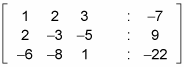
Now take a look at the goals of Gaussian elimination in order to complete the following steps to solve this matrix:

1. Complete the first goal: to get 1 in the upper-left corner.

   You already have it!

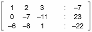
2. Complete the second goal: to get 0s underneath the 1 in the first column.

   You need to use the combo of two matrix operations together here. Here's what you should ask: "What do I need to add to row two to make a 2 become a 0?" The answer is –2.

   This step can be achieved by multiplying the first row by –2 and adding the resulting row to the second row. In other words, you perform the operation

   

   which produces this new row:

   1. (–2 –4 –6 : 14) + (2 –3 –5 : 9) = (0 –7 –11: 23)

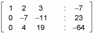
   You now have this matrix:

   

3. In the third row, get a 0 under the 1.

   To do this step, you need the operation

   

   With this calculation, you should now have the following matrix:

   

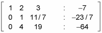
4. Get a 1 in the second row, second column.

   To do this step, you need to multiply by a constant; in other words, multiply row two by the appropriate reciprocal:

   

   This calculation produces a new second row:

   

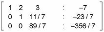
5. Get a 0 under the 1 you created in row two.

   Back to the good old combo operation for the third row:

   

   Here's yet another version of the matrix:

   

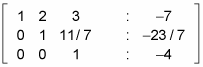
6. Get another 1, this time in the third row, third column.

   Multiply the third row by the reciprocal of the coefficient to get a 1:

   

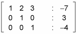
   You've completed the main diagonal after doing the math:

   

1. Get a 0 in row two, column three.

   Multiplying row three by the constant –11/7 and then adding rows two and three

   

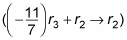
   gives you the following matrix:

   

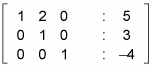
2. Get a 0 in row one, column three.

   The operation

   

   gives you the following matrix:

   

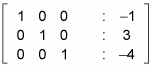
3. Get a 0 in row one, column two.

   Finally, the operation

   

   gives you this matrix: