the standard normal tables requires you to convert
to a standard normal random variable.
The standard normal distribution is the special case where the mean
equals 0, and the standard deviation
equals 1.
For any normally distributed random variable X with a mean
and a standard deviation
you find the corresponding standard normal random variable (Z) with the following equation:
For the sampling distribution of
the corresponding equation is

As an example, say that there are 10,000 stocks trading each day on a regional stock exchange. It's known from historical experience that the returns to these stocks have a mean value of 10 percent per year, and a standard deviation of 20 percent per year.
An investor chooses to buy a random selection of 100 of these stocks for his portfolio. What's the probability that the mean rate of return among these 100 stocks is greater than 8 percent?
The investor's portfolio can be thought of as a sample of stocks chosen from the population of stocks trading on the regional exchange. The first step to finding this probability is to compute the moments of the sampling distribution.
-
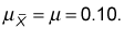
Compute the mean:
-
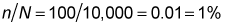
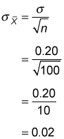
Determine the standard error: This calculation is a little trickier because the standard error depends on the size of the sample relative to the size of the population. In this case, the sample size (n) is 100, while the population size (N) is 10,000. So you first have to compute the sample size relative to the population size, like so:
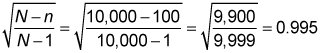
Because 1 percent is less than 5 percent, you don't use the finite population correction factor to compute the standard error. Note that in this case, the value of the finite population correction factor is:
And because the finite population correction factor isn't needed in this case, the standard error is computed as follows:
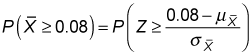
To determine the probability that the sample mean is greater than 8 percent, you must now convert the sample mean into a standard normal random variable using the following equation:

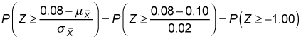
To compute the probability that the sample mean is greater than 8 percent, you apply the previous formula as follows:
Because
these values are substituted into the previous expression as follows:
You can calculate this probability by using the properties of the standard normal distribution along with a standard normal table such as this one.
| Z | 0.00 | 0.01 | 0.02 | 0.03 |
|---|---|---|---|---|
| –1.3 | 0.0968 | 0.0951 | 0.0934 | 0.0918 |
| –1.2 | 0.1151 | 0.1131 | 0.1112 | 0.1093 |
| –1.1 | 0.1357 | 0.1335 | 0.1314 | 0.1292 |
| –1.0 | 0.1587 | 0.1562 | 0.1539 | 0.1515 |
(one standard deviation below the mean) as
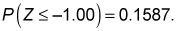
You find the probability from the table with these steps:
-
Locate the first digit before and after the decimal point (–1.0) in the first (Z) column.
-
Find the second digit after the decimal point (0.00) in the second (0.00) column.
-
See where the row and column intersect to find the probability:
Due to the symmetry of the standard normal distribution, the probability that Z is greater than or equal to a negative value equals one minus the probability that Z is less than or equal to the same negative value.
For example,
This is because
are complementary events. This means that Z must either be greater than or equal to –2 or less than or equal to –2. Therefore,
This is true because the occurrence of one of these events is certain, and the probability of a certain event is 1.
After algebraically rewriting this equation, you end up with the following result:
For the portfolio example,
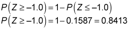
The result shows that there's an 84.13 percent chance that the investor's portfolio will have a mean return greater than 8 percent.