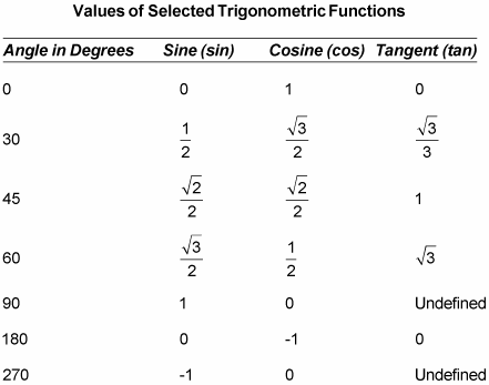
Commonly used values of selected trig functions
When performing transformations in trig functions, such as rotations, you need to use the numerical values of these functions. Here are some of the more commonly used angles.
How to meet vector space requirements
In linear algebra, a set of elements is termed a vector space when particular requirements are met. For example, let a set consist of vectors u, v, and w. Also let k and l be real numbers, and consider the defined operations of ⊕ and ⊗. The set is a vector space if, under the operation of ⊕, it meets the following requirements:
-
Closure. u ⊕ v is in the set.
-
Commutativity. u ⊕ v = v ⊕ u.
-
Associativity. u ⊕ (v ⊕ w) = (u ⊕ v) ⊕ w.
-
An identity element 0. u ⊕ 0 = 0 ⊕ u = u for any element u.
-
An inverse element −u. u ⊕ −u = −u ⊕ u = 0
Under the operation of ⊗, the set is a vector space if it meets the following requirements:
-
Closure. k ⊗ u is in the set.
-
Distribution over a vector sum. k ⊗ (u ⊕ v) = k ⊗ u ⊕ k⊗ v.
-
Distribution over a scalar sum. (k + l) ⊗ u = k ⊗u ⊕ l ⊗ u.
-
Associativity of a scalar product. k ⊗ (l ⊗ u) = (kl) ⊗ u.
-
Multiplication by the scalar identity. 1 ⊗ u = u.
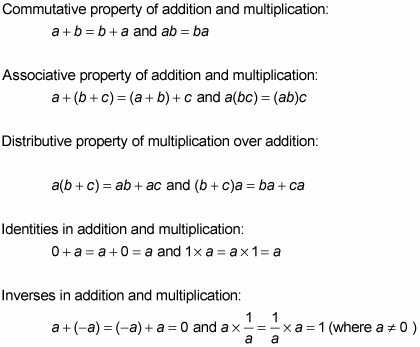
Algebraic properties you should know
You can use a number of properties when working with linear algebraic expressions, including the commutative, associative, and distributive properties of addition and multiplication, as well as identities and inverses in addition and multiplication:
Calculator commands for linear algebra
Graphing calculators are wonderful tools for helping you solve linear algebra processes; they allow you to drain battery power rather than brain power. Since there is a wide variety of graphing calculators out there, the following are general instructions for help with linear algebra that apply to most graphing calculators:
To solve systems of equations by graphing:
-
1. Write each equation in y = mx + b form.
-
2. Insert equations in the y-menu.
-
3. Graph the lines.
-
4. Use the Intersection tool to get the answer.
To add or subtract matrices:
-
1. Insert the elements into the matrices A and B.
-
2. With a new screen, press [A] + [B] or [A] – [B], and press Enter.
To multiply by a scalar:
-
1. Insert the elements into the matrix A.
-
2. With a new screen, press the scalar and multiply: k * [A], and press Enter.
To multiply two matrices together:
-
1. Insert the elements into the matrices A and B.
-
2. With a new screen, press [A] * [B], and press Enter.
To switch rows:
-
1. Insert the elements into a matrix.
-
2. Use row swap: rowSwap ([matrix name], first row, second row), and press Enter.
To add two rows together:
-
1. Insert the elements into a matrix.
-
2. Use row addition: “row +”, ([matrix name], row to be added to target row, target row), and press Enter.
To add the multiple of one row to another:
-
1. Insert the elements into a matrix.
-
2. Use row sum–of–multiple: “*row +”, (multiplier, [matrix name], row being multiplied, target row having multiple added to it), and press Enter.
To multiply a row by a scalar:
-
1. Insert the elements into a matrix.
-
2. Use row multiple: “*row” (multiplier, [matrix name], row), and press Enter.
To create an echelon form:
-
1. Insert the elements into a matrix.
-
2. Use row–echelon form: ref ([matrix name]) or reduced row-echelon form: rref ([matrix name]), and press Enter.
To raise a matrix to a power:
-
1. Insert the elements into a matrix.
-
2. Use the caret operation with power, p: [matrix name] ^ p, and press Enter.
To find inverses:
-
1. Insert the elements into a matrix.
-
2. Use the reciprocal operation, x−1: [matrix name]−1, and press Enter.
To solve systems of linear equations:
(This only works when the system has a single solution; it fails when the matrix A is singular.)
-
1. Write each equation with the variables in the same order and the constant on the other side of the equation sign.
-
2. Create a matrix A, whose elements are the coefficients of the variables.
-
3. Create a matrix B, whose elements are the constants.
-
4. Press, A−1 * B, and press Enter.
The resulting vector has the values of the variables, in order.