Matrices are the perfect tool for solving systems of equations (the larger the better). Fortunately, you can work with matrices on your TI-84 Plus. All you need to do is decide which method you want to use.
A–1*B method of solving a system of equations
What do the A and B represent? The letters A and B are capitalized because they refer to matrices. Specifically, A is the coefficient matrix and B is the constant matrix. In addition, X is the variable matrix. No matter which method you use, it's important to be able to convert back and forth from a system of equations to matrix form.

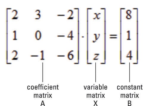
Here’s a short explanation of where this method comes from. Any system of equations can be written as the matrix equation, A * X = B. By pre-multiplying each side of the equation by A–1 and simplifying, you get the equation X = A–1 * B.
Using your calculator to find A–1 * B is a piece of cake. Just follow these steps:
Enter the coefficient matrix, A.
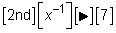
Press [ALPHA][ZOOM] to create a matrix from scratch or press [2nd][x–1] to access a stored matrix. See the first screen.
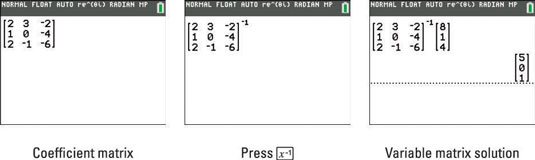
Press [x–1] to find the inverse of matrix A.
See the second screen.
Enter the constant matrix, B.
Press [ENTER] to evaluate the variable matrix, X.
The variable matrix indicates the solutions: x = 5, y = 0, and z = 1. See the third screen.
If the determinant of matrix A is zero, you get the ERROR: SINGULAR MATRIX error message. This means that the system of equations has either no solution or infinite solutions.
Augmenting matrices method to solve a system of equations
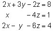
Augmenting two matrices enables you to append one matrix to another matrix. Both matrices must be defined and have the same number of rows. Use the system of equations to augment the coefficient matrix and the constant matrix.
To augment two matrices, follow these steps:
To select the Augment command from the MATRX MATH menu, press
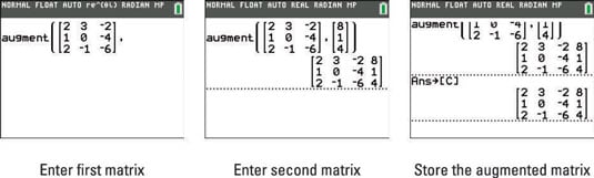
Enter the first matrix and then press [,] (see the first screen).
To create a matrix from scratch, press [ALPHA][ZOOM]. To access a stored matrix, press [2nd][x–1].
Enter the second matrix and then press [ENTER].
The second screen displays the augmented matrix.
Store your augmented matrix by pressing
The augmented matrix is stored as [C]. See the third screen.
Systems of linear equations can be solved by first putting the augmented matrix for the system in reduced row-echelon form. The mathematical definition of reduced row-echelon form isn’t important here. It’s simply an equivalent form of the original system of equations, which, when converted back to a system of equations, gives you the solutions (if any) to the original system of equations.
To find the reduced row-echelon form of a matrix, follow these steps:
To scroll to the rref( function in the MATRX MATH menu, press

and use the up-arrow key. See the first screen.
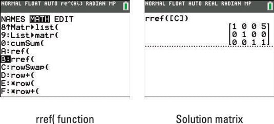
Press [ENTER] to paste the function on the Home screen.
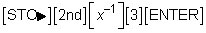
Press [2nd][x–1] and press [3] to choose the augmented matrix you just stored.
Press [ENTER] to find the solution.
See the second screen.
To find the solutions (if any) to the original system of equations, convert the reduced row-echelon matrix to a system of equations:
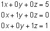
As you see, the solutions to the system are x = 5, y = 0, and z = 1. Unfortunately, not all systems of equations have unique solutions like this system. Here are examples of the two other cases that you may see when solving systems of equations:
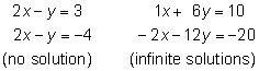
See the reduced row-echelon matrix solutions to the preceding systems in the first two screens.
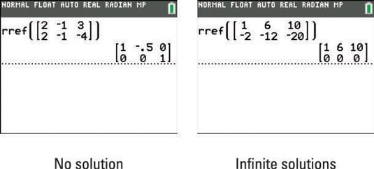
To find the solutions (if any), convert the reduced row-echelon matrices to a system of equations:
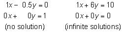
Because one of the equations in the first system simplifies to 0 = 1, this system has no solution. In the second system, one of the equations simplifies to 0 = 0. This indicates the system has an infinite number of solutions that are on the line x + 6y = 10.