Multiple-input production functions allow you to account for more complexity in your firm’s decision-making processes. Although single-input production functions are useful for illustrating many concepts, usually, they’re too simplistic to represent a firm’s production decision. In other words, you’re dealing with two or more variable inputs.
Consider the production function q = f(L,K), which indicates the quantity of output produced is a function of the quantities of labor, L, and capital, K, employed. The specific form of this function may be the following Cobb-Douglas function
Production isoquants: All input combinations are equal
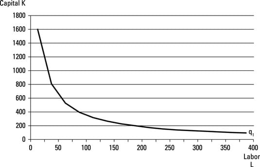
The relationship between labor, capital, and the quantity of output produced in the previous equation is graphically described by using a production isoquant. A production isoquant shows all possible combinations of two inputs that produce a given quantity of output.
The curve labeled q1 represents all combinations of capital and labor that produce 3,200 units of output.
Marginal product
Marginal product is the change in total product that occurs given one additional unit of an input. With a production isoquant, the amount of output you gain from using one more unit of labor is exactly offset by the amount of output you lose by using less capital.
Every input combination on the production isoquant produces the same level of output — output is constant. Capital can change by more or less than one unit. What is critical is that total product remains constant as you increase labor and decrease capital.
Marginal rate of technical substitution
The marginal rate of technical substitution measures the change in the quantity of the input on the vertical axis of the diagram that’s necessary per one-unit change of the input on the horizontal axis of the diagram in order for total product to remain constant.
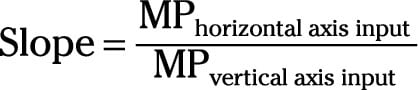
That’s too technical of a definition, so remember this instead — the marginal rate of technical substitution is simply the production isoquant’s slope. The production isoquant’s slope equals the marginal product of the input on the horizontal axis divided by the marginal product the input on the vertical axis.
Isocost curves: All input combinations cost the same
An important factor in your production decision is how much the inputs cost. If an additional worker (unit of labor) costs less than an additional unit of capital, but the worker produces the same quantity of output as the capital, it’s a good deal to hire the additional worker. So, you need to add cost to your decision-making process.
The isocost curve illustrates all possible combinations of two inputs that result in the same level of total cost. The isocost curve is presented as an equation. For a situation with two inputs — labor and capital — the isocost curve’s equation is
In this equation, C is a constant level of cost, pL is the price of labor, L is the quantity of labor employed, pK is the price of capital, and K is the quantity of capital employed.
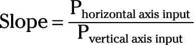
On a graph, the isocost curve’s slope equals the price of the input on the horizontal axis divided by the price of the vertical axis input.
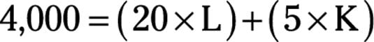
Assume your total cost is $4,000 a day, and labor costs $20 per hour, and capital costs $5 per machine-hour. Given this information, your isocost curve equation is
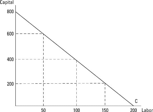
Some possible combinations of labor and capital you can employ for a total cost of $4,000 are 50 hours of labor and 600 machine-hours of capital, 100 hours of labor and 400 machine-hours of capital, and 150 hours of labor and 200 machine hours of capital. Any combination of labor and capital that results in total cost being $4,000 would be on the same — $4,000 — isocost curve.
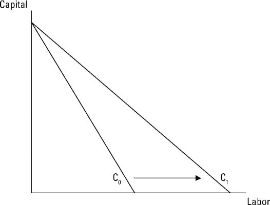
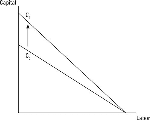
Changes in input prices shift the isocost curve. If the input on the horizontal axis becomes cheaper, the isocost curve rotates out on that axis. If the input on the vertical axis becomes cheaper, the isocost curve rotates. More expensive inputs cause shifts in the opposite direction.
How to minimize costs
In order to maximize profits, you must produce your output at the lowest possible cost.
The costs of producing a given quantity of output are minimized at the point where the production isoquant is just tangent — or, in other words, just touching — the isocost curve. This point is illustrated as point A. The cost-minimizing combination of labor and capital are the quantities L0 and K0.
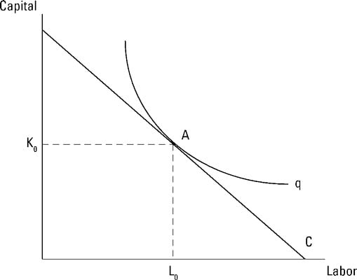
Now comes the easy part. At the point where you minimize costs, the production isoquant and isocost curve are tangent. This means the slopes of these two curves are equal. Therefore
Or, if you rearrange that equation
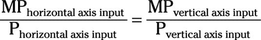
Thus, you minimize costs when the marginal product per dollar spent on each input is equal for all inputs. And this holds true no matter how many inputs you use!
Economists call the preceding concept the least cost criterion, and it’s an application of the equimarginal principle. To produce goods with the lowest possible production cost, you equate the marginal product per dollar spent.