In the long run, none of your inputs are fixed. In managing your firm, you can choose any input combination to produce a given quantity of output. This decision ultimately leads to the selection of some inputs that become fixed after their initial selection.
For example, when considering whether or not to produce the Saturn, General Motors could have chosen a variety of configurations for the factory. Each configuration General Motors evaluated had its own short-run average-total-cost curve.
After a configuration was chosen, it became a fixed input, and General Motors subsequently operated on the short-run average-total-cost curve associated with that configuration. Therefore, General Motors’ long-run decision amounted to choosing the best possible short-run average-total-cost curve from a variety of possibilities.
How to put costs in the envelope curve
Because there are no fixed inputs in the long run, the long-run total cost function doesn’t have a constant. Therefore, if you decide to produce zero units of output in the long run, your total cost equals zero.
The long-run average-total-cost curve is derived by dividing the long-run total-cost function by the quantity of output. Another way to view long-run average total cost is to keep in mind that a short-run average-total-cost curve is associated with a given level of fixed inputs. If you choose a different level of fixed inputs, you get a different short-run average-total-cost curve.
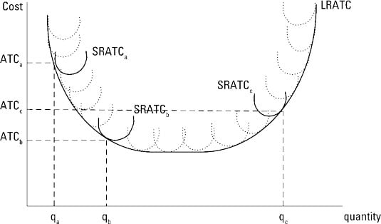
The long-run average-total-cost curve reflects the set of fixed inputs that yields the lowest possible cost of producing each output level. Therefore, the long-run average-total-cost curve links the short-run average-total-cost curves associated with the minimum cost of producing any output level. Or, the long-run average-total-cost curve is the envelope that holds all the short-run possibilities.
The illustration shows a long-run average-total-cost curve. The lowest per-unit cost associated with producing the output level qb is ATCb. This cost results when the fixed inputs associated with the short-run average-total-cost curve SRATCb are chosen.
Similarly, the fixed inputs associated with SRATCa result in the production of qa with the lowest per-unit cost ATCa, and the fixed inputs associated with SRATCc result in the production of qc with the lowest per-unit cost ATCc.
Economies of scale
Economies of scale exist when long-run average total cost decreases as the quantity of output produced increases. Economies of scale result from many different factors, including increasing returns to scale, quantity discounts on input prices, and the ability to spread management and overhead costs over a larger quantity of output.
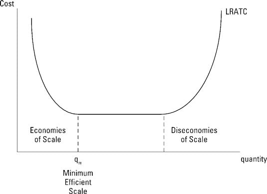
In the illustration, economies of scale are associated with the downward-sloping portion of the long-run average-total-cost curve.
How to avoid diseconomies of scale
Diseconomies of scale occur when long-run average total cost increases as the quantity of output produced increases. Diseconomies of scale may result from decreasing returns to scale or managerial limitations resulting from the firm’s large size. Larger firms become increasingly complex, making it more difficult to coordinate necessary activities.
Diseconomies of scale correspond to the upward-sloping segment of the long-run average-total-cost curve.
Diseconomies of scale indicate that your cost per unit increases as you produce more output. This isn’t just higher per-unit cost for the additional units — it’s higher cost for all units.
How to identify the minimum efficient scale
The minimum efficient scale is the output level at which economies of scale cease. Therefore, it’s the smallest output quantity that results in minimum cost per unit. Any production scale below this minimum efficient scale is at a disadvantage relative to other scales, because its per-unit production costs are higher than this.
In the illustration, the minimum efficient scale occurs at the output level qm.
Estimates of long-run average total cost for various industries typically indicate the presence of economies of scale at small output levels — long-run average total cost is decreasing for these output levels.
After economies of scale are exhausted, however, research has generally indicated that long-run average total cost becomes constant, implying that the long-run average-total-cost curve is horizontal. Therefore, diseconomies of scale, or increasing long-run average total cost, is rarely observed in actual commodity production.