Oligopolies commonly compete by trying to steal market share from one another. Thus, rather than compete by lowering price — the kinked demand curve indicates that this tactic doesn’t work because everyone lowers price — firms often compete on the other factor that directly affects profit — the quantity of the good they sell.
The Cournot model is used when firms produce identical or standardized goods and don’t collude. Each firm assumes that its rivals make decisions that maximize profit.
The Cournot duopoly model offers one view of firms competing through the quantity produced. Duopoly means two firms, which simplifies the analysis. The Cournot model assumes that the two firms move simultaneously, have the same view of market demand, have good knowledge of each other’s cost functions, and choose their profit-maximizing output with the belief that their rival chooses the same way.
With all these assumptions, you may wonder why not just assume the right answer. Unfortunately, it doesn’t work that way. On the other hand, you may think that these assumptions are unrealistic. However, research has shown that decision-makers operating in the same market over an extended period of time tend to have similar views of market demand and good knowledge of one another’s cost structure.
Given these assumptions, one firm reacts to what it believes the other firm will produce. In other words, if firm B produces qB of output, what quantity should firm A produce? The Cournot reaction function describes the relationship between the quantity firm A produces and the quantity firm B produces. Here’s how it works.
The market demand curve faced by Cournot duopolies is:
where QD is the market quantity demanded and P is the market price in dollars.
Assuming firm A has a constant marginal cost of $20 and firm B has a constant marginal cost of $34, the reaction function for each firm is derived by using the following steps:
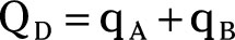
Note that the market quantity demand, QD, must be jointly satisfied by firms A and B.
Thus,
Substituting the equation in Step 1 for QD in the market demand curve yields

For firm A, total revenue equals price multiplied by quantity.

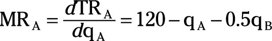
Firm A’s marginal revenue is determined by taking the derivative of total revenue, TRA, with respect to qA.
Remember to treat qB as a constant because firm A can’t change the quantity of output produced by firm B.
Firm A maximizes profit by setting its marginal revenue equal to marginal cost.
Firm A’s marginal cost equals $20.

Rearranging the equation in Step 5 to solve for qA gives firm A’s reaction function.

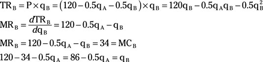
Repeat Steps 3 through 6 to determine firm B’s reaction function.
Remember that firm B’s marginal cost equals $34.
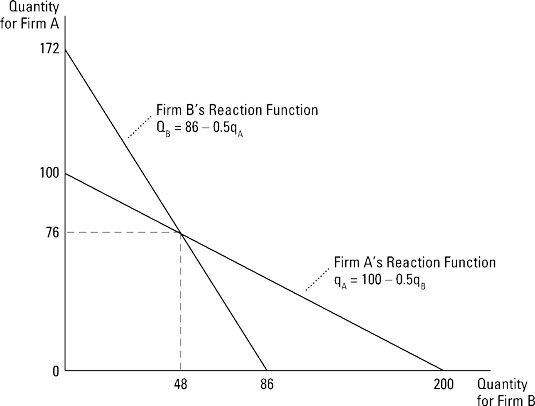
Substituting firm B’s reaction function for qB in firm A’s reaction function enables you to solve for qA.
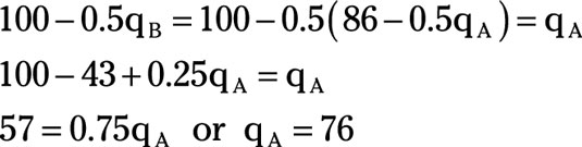
Substituting qA = 76 in firm B’s reaction function enables you to solve for qB.

Thus, in the profit maximizing Cournot duopolist, firm A, produces 76 units of output while firm B produces 48 units of output.
In the Cournot duopoly model, both firms determine the profit-maximizing quantity simultaneously.
In the last example, firms A and B had different marginal costs. If the firms have the same marginal costs (MCA = MCb), each firm produces half the market output.