


You can use the column sorting capability in Excel 2013 to change the order of the fields in a data list without having to resort to cutting and pasting various columns.
When you sort the fields in a data list, you add a row at the top of the list that you define as the primary sorting level. The cells in this row contain numbers (from 1 to the number of the last field in the data list) that indicate the new order of the fields.
You can’t sort data you’ve formally formatted as a data table until you convert the table back into a normal cell range because the program won’t recognize the row containing the column’s new order numbers as part of the table on which you can perform a sort.
In this example, to get around the problem, you take the following steps:
Click a cell in the data table and then click the Convert to Range command button on the Design tab of the Table Tools contextual tab.
Excel displays an alert dialog box asking you if you want to convert the table to a range.
Click the Yes button in the alert dialog box to do the conversion.
Select all the records in the Personnel data list along with the top row containing the numbers on which to sort the columns of the list as the cell selection.
In this case, you select the cell range A1:H20 as the cell selection.
Click the Sort command button on the Data tab (or press Alt+ASS).
Excel opens the Sort dialog box. You can also open the Sort dialog box by selecting Custom Sort from the Sort & Filter button’s drop-down list or by pressing Alt+HSU.
Click the Options button in the Sort dialog box.
Excel opens the Sort Options dialog box.
Select the Sort Left to Right option button and then click OK.
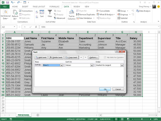
Click Row 1 in the Row drop-down list in the Sort dialog box.
The Sort On drop-down list box should read Values, and the Order drop-down list box should read Smallest to Largest.
Click OK to sort the data list using the values in the top row of the current cell selection.
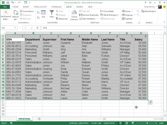
Excel sorts the columns of the Personnel data list according to the numerical order of the entries in the top row (which are now in a 1-to-8 order). Now, you can get rid of the top row with these numbers.
Select the cell range A1:H1 and then click the Delete button on the Home tab.
Excel deletes the row of numbers and pulls up the Personnel data list so that its row of field names is now in row 1 of the worksheet. Now, all that’s left to do is to reformat the Personnel data list as a table again so that Excel adds AutoFilter buttons to its field names and the program dynamically keeps track of the data list’s cell range as it expands and contracts.
Click the Format as Table command button on the Home tab (or press Alt+HT) and then click a table style from the Light, Medium, or Dark section of its gallery.
Excel opens the Format As Table dialog box and places a marquee around all the cells in the data list.
Make sure that the My Table Has Headers check box has a check mark in it and that all the cells in the data list are included in the cell range displayed in the Where Is the Data for Your Table text box before you click OK.
The personnel data list’s fields are sorted according to the values in the first row. After sorting the data list, you then delete this row and modify the widths of the columns to suit the new arrangement and reformat the list as a table before you save the worksheet.
