You may have a table in Excel 2013 in which you need to perform a two-way lookup, whereby a piece of data is retrieved from the Lookup table based on looking up a value in the top row (with the table’s column headings) and a value in the first column (with the table’s row headings).
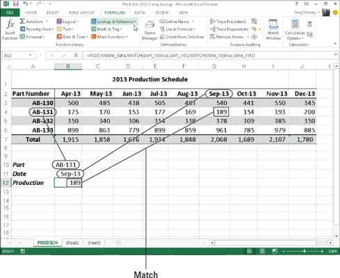
The figure illustrates a situation in which you would use two values, the production date and the part number, to look up the expected production. In the 2013 Production Schedule table, the production dates for each part form the column headings in the first row of the table, and the part numbers form the row headings in its first column of the table.

To look up the number of the part scheduled to be produced in a particular month, you need to the use the MATCH function, which returns the relative position of a particular value in a cell range or array. The syntax of the MATCH function is as follows:
MATCH(lookup_value,lookup_array,[match_type])
The lookup_value argument is, of course, the value whose position you want returned when a match is found, and the lookup_array is the cell range or array containing the values that you want to match. The optional match_type argument is the number 1, 0, or –1, which specifies how Excel matches the value specified by the lookup_value argument in the range specified by the lookup_array argument:
Use match_type 1 to find the largest value that is less than or equal to the lookup_value. Note that the values in the lookup_array must be placed in ascending order when you use the 1 match_type argument. (Excel uses this type of matching when the match_type argument is omitted from the MATCH function.)
Use match_type 0 to find the first value that is exactly equal to the lookup_value. Note that the values in the lookup_array can be in any order when you use the 0 match_type argument.
Use match_type –1 to find the smallest value that is greater than or equal to the lookup_value. Note that the values in the lookup_array must be placed in descending order when you use the –1 match_type argument.
In addition to looking up the position of the production date and part number in the column and row headings in the Production Schedule table, you need to use an INDEX function, which uses the relative row and column number position to return the number to be produced from the table itself.
The INDEX function follows two different syntax forms: array and reference. You use the array form when you want a value returned from the table (as you do in this example), and you use the reference form when you want a reference returned from the table.
The syntax of the array form of the INDEX function is as follows:
INDEX(array,[row_num],[col_num])
The syntax of the reference form of the INDEX function is as follows:
INDEX(reference,[row_num],[col_num],[area_num])
The array argument of the array form of the INDEX function is a range of cells or an array constant that you want Excel to use in the lookup. If this range or constant contains only one row or column, the corresponding row_num or col_num arguments are optional.
If the range or array constant has more than one row or more than one column, and you specify both the row_num and the col_num arguments, Excel returns the value in the array argument that is located at the intersection of the row_num argument and the col_num argument.
For the MATCH and INDEX functions in the example, the following range names were assigned to the following cell ranges:
table_data to the cell range A2:J6 with the production data plus column and row headings
part_list to the cell range A2:A6 with the row headings in the first column of the table
date_list to the cell range A2:J2 with the column headings in the first row of the table
part_lookup to cell B10 that contains the name of the part to look up in the table
date_lookup to cell B11 that contains the name of the production date to look up in the table
As the figure shows, cell B12 contains a rather long and — at first glance — complex formula using the range names outlined previously and combining the INDEX and MATCH functions:
=INDEX(table_data,MATCH(part_lookup,part_list),MATCH(date_lookup,date_list))

