Running multiple scenarios is a very important part of financial modeling — some would say it’s the whole point of financial modeling — because it allows the user to gauge the different outcomes if certain assumptions end up being different. Because no one can see into the future and assumptions invariably end up being wrong, being able to see what happens to the outputs when the main assumption drivers are changed is important.
Because you’ve built this integrated financial model such that all the calculations are linked either to input assumption cells, or to other parts of the financial statements, any changes in assumptions should flow nicely throughout the model. The proof is in the pudding, however.
Entering your scenario assumptions
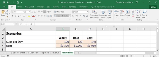
Going back now to the Assumptions worksheet, you believe that the main drivers of profitability for your cafe will be the average number of cups you sell per day and the rent you’ll pay. You believe that reducing cups sold per day by 20 cups and increasing rent by 10 percent is a reasonable worst-case scenario, and increasing cups sold per day by 20 cups and reducing rent by 10 percent is a reasonable best-case scenario.At the very top of the Assumptions worksheet, enter the scenario input assumptions.
Building a drop-down box
You’ve decided on your scenario assumptions, so now you need to build a drop-down box, which is going to drive your scenario analysis. You have a full, working financial model, so you want the ability to easily switch between your scenarios to see how the outputs change in real time. You can put the scenario drop-down box on either of the financial statements, but for this example you’ll put it at the top of the income statement.Follow these steps:
- Go to the IS Cash Flow worksheet and select cell B1.
- Select Data Validation in the Data Tools section of the Data Ribbon.
The Data Validation dialog box appears.
- From the Allow drop-down list, select List.
You could type the words Best, Base, and Worst directly into the field, but it’s best to link it to the source in case you misspell a value.
- In the Source field, type = and then click the Assumptions worksheet, and highlight the scenario names Worst, Base, Best.
Your formula in the Source field should now be =Assumptions!$B$2:$D$2.
- Click OK.
- Go back to cell B1 on the IS Cash Flow worksheet, and test that the drop-down box is working as expected and gives the options Best, Base, and Worst.
- Set the drop-down box to Base for now.
Building the scenario functionality
You need to edit your input assumptions for number of cups sold per day and monthly rent so that as the drop-down box on the IS Cash Flow worksheet changes, the input assumptions change to the corresponding scenario. For example, when Best has been selected on the IS Cash Flow worksheet, the value in cell B9 on the Assumptions worksheet should be 140, and the value in cell B23 should be $1,080. This should be done using a formula.Often, many different functions will achieve the same or similar results. Which function you use is up to you as the financial modeler, but the best solution will be the one that performs the required functionality in the cleanest and simplest way, so that others can understand what you’ve done and why.
In this case, there are several options you could use: a HLOOKUP, a SUMIF, or an IF statement. The IF statement, being a nested function, is the most difficult to build and is less scalable. If the number of scenario options increase, the IF statement option is more difficult to expand. In this instance, I have chosen to use the HLOOKUP with these steps.Follow these steps:
- Select cell B9 and press the Insert Function button on the Formulas tab or next to the formula bar.
- Search for HLOOKUP, press Go, and click OK.
The HLOOKUP dialog box appears.
- Click the Lookup_value field, and select the drop-down box on the IS Cash Flow worksheet.
This is the criteria that drives the HLOOKUP.
- Press F4 to lock the cell reference.
In the Table_array field, you need to enter the array you’re using for the HLOOKUP. Note that your criteria must appear at the top of the range.
- Select the range that is the scenario table at the top — in other words, B2:D4 — and the press F4 to lock the cell references.
The cell references will change to $B$2:$D$4.
- In the Row_index_num field, enter the row number, 2.
- In the Range_lookup field, enter a zero or false, because you’re looking for an exact match.
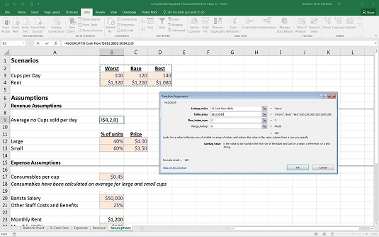
- Check that your dialog box looks the same as the image below.
- Click OK.
The formula in cell B9 is =HLOOKUP(‘IS Cash Flow’!B1,$B$2:$D$4,2,0) with the calculated result of 120.
- Perform the same action in cell B23 with the formula =HLOOKUP(‘IS Cash Flow’!$B$1,$B$2:$D$4,3,0).
Instead of re-creating the entire formula again, simply copy the formula from cell B9 to cell B23 and change the row reference from 2 to 3. Copying the cell will change the formatting of the number, so you’ll need to change the currency symbol back to $ again.
- Go back to the IS Cash Flow worksheet and change the drop-down to Best.
Check that your assumptions for average number of cups sold per day and monthly rent on the Assumptions worksheet have changed accordingly. Cups will have changed to 140 and rent to $1,080.
Now, the important test is to see if the balance sheet still balances!
- Go back to the Balance Sheet worksheet and make sure that your error check is still zero.
- Test the drop-down again by changing it to Worst.
Cups will have changed to 100 and rent will be $1,320. Check the error check on the Balance Sheet worksheet again.
Congratulations! Your entirely integrated financial model, together with scenario analysis, is now complete! You can download a copy of the completed model in File 1002.xlsx.