How to Add Math Symbols in MATLAB

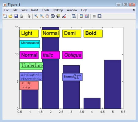
Displaying a fraction onscreen doesn’t always include a numeric fraction; it could be a formula that requires that sort of presentation. Whatever your need, you can display fractions whenever needed. However, to do that, you must use the LaTeX interpreter. This means that your formatting options are limited and that the output won’t necessarily reflect the formatting choices you normally make when using MATLAB.

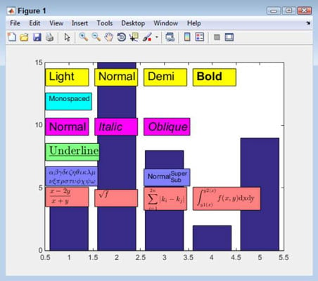
The fraction requires use of a LaTeX display style that you access using $displaystylefrac. The fraction itself appears in two curly brackets, such as {1}{2} for the symbol 1/2. The entry ends with another dollar sign ($). To see how fractions work with something a little more complex, type TBox12 = annotation(‘textbox’, [.13, .3, .14, .075], ‘String’, ‘$displaystylefrac{x-2y}{x+y}$’, ‘BackgroundColor’, [1, .5, .5], ‘Interpreter’, ‘latex’); and press Enter.

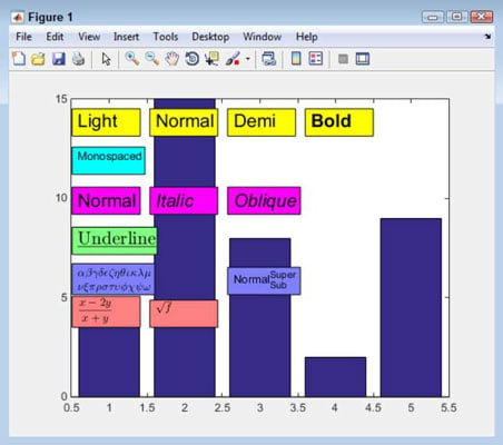
MATLAB makes displaying a square root symbol easy. However, getting the square root symbol the right size and with the bar extended over the expression whose root is being taken requires LaTeX.

As with many LaTeX commands, you enclose the string that you want to format in a pair of dollar signs ($). The function used to perform the formatting is sqrt{}, and the value that you want to place within the square root symbol appears within the curly brackets.

To see the square root symbol in action, type TBox13 = annotation(‘textbox’, [.29, .3, .14, .075], ‘String’, ‘$sqrt{f}$’, ‘BackgroundColor’, [1, .5, .5], ‘Interpreter’, ‘latex’); and press Enter. The variable f will appear in the square root symbol.

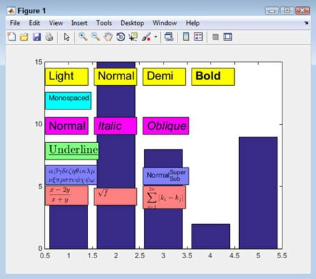
Displaying a summation formula complete with sigma and the upper and lower limit involves using LaTeX with the sum function. You supply all three elements of the display in a single statement: the lower limit first, the upper limit second, and the expression third. Each element appears in separate curly brackets.

The lower limit is preceded by the underscore used for subscripts and the upper limit is preceded by the caret used for superscripts. The entire statement appears within dollar signs ($), as is normal for LaTeX. However, in this particular case, you must include a second set of dollar signs or the expression doesn’t appear correctly onscreen. (The upper and lower limits don’t appear in the correct places.)

To see how summation works, type TBox14 = annotation(‘textbox’, [.45, .285, .14, .1], ‘String’, ‘$$sum_{i=1}^{2n}{|k_i-k_j|}$$’, ‘BackgroundColor’, [1, .5, .5], ‘Interpreter’, ‘latex’); and press Enter. Notice the use of the double dollar signs in this case. In addition, be sure to include both the underscore and caret, as shown.

To display a definite integral, you use the LaTeX int function, along with the d function for the slices. The int function accepts three inputs: two for the interval and the third for the function. In many respects, the format is the same as that used for summation.

The beginning of the interval relies on the superscript caret character, while the ending of the interval relies on the subscript underscore character. You must enclose the entire command within double dollar signs ($$) or else the formatting of the superscript and subscript will fail.

To see how to create an integral, type TBox15 = annotation(‘textbox’, [.61, .285, .22, .1], ‘String’, ‘$$int_{y1(x)}^{y2(x)}{f(x,y)}d{dx}d{dy}$$’, ‘BackgroundColor’, [1, .5, .5], ‘Interpreter’, ‘latex’); and press Enter. Notice that the two slices come after the int function and that each slice appears in its own d function.

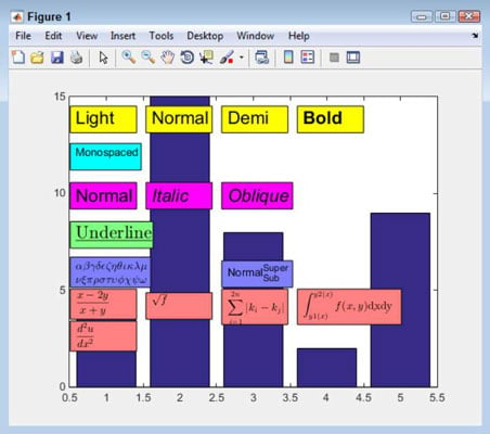
When creating a derivative, you use LaTeX to define a combination of a fraction with superscripts. So, in reality, you’ve already created a derivative in the past — at least in parts. To see how a derivative works, type TBox16 = annotation(‘textbox’, [.13, .21, .14, .085], ‘String’, ‘$displaystylefrac{d^2u}{dx^2}$’, ‘BackgroundColor’, [1, .5, .5], ‘Interpreter’, ‘latex’); and press Enter.