
For example, each pixel of a picture file could consist of three 32-bit fields. Knowing that each field is 32 bits is up to you. A header at the beginning of the file may provide clues about interpreting the file, but even so, it’s up to you to know how to interact with the file using the right package or library.
You use Scikit-image here. It’s a Python package dedicated to processing images, picking them up from files, and handling them using NumPy arrays. By using Scikit-image, you can obtain all the skills needed to load and transform images for any machine learning algorithm. This package also helps you upload all the necessary images, resize or crop them, and flatten them into a vector of features in order to transform them for learning purposes.
Scikit-image isn’t the only package that can help you deal with images in Python. There are also other packages, such as the following:
- scipy.ndimage: Allows you to operate on multidimensional images
- Mahotas: A fast C++ based processing library
- OpenCV: A powerful package that specializes in computer vision
- ITK: Designed to work on 3D images for medical purposes
from skimage.io import imread
from skimage.transform import resize
from matplotlib import pyplot as plt
import matplotlib.cm as cm
%matplotlib inline
example_file = ("http://upload.wikimedia.org/" +
"wikipedia/commons/7/7d/Dog_face.png")
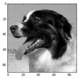
image = imread(example_file, as_grey=True)
plt.imshow(image, cmap=cm.gray)
plt.show()
The code begins by importing a number of libraries. It then creates a string that points to the example file online and places it in example_file. This string is part of the imread() method call, along with as_grey, which is set to True. The as_grey argument tells Python to turn any color images into grayscale. Any images that are already in grayscale remain that way.
After you have an image loaded, you render it. The imshow() function performs the rendering and uses a grayscale color map. The show() function actually displays image for you.
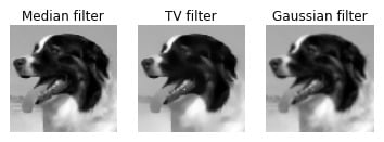
Sometimes images aren’t perfect; they can present noise or other granularity. You must smooth the erroneous and unusable signals. Filters can help you achieve that smoothing without hiding or modifying important characteristics of the image, such as the edges. If you’re looking for an image filter, you can clean up your images using the following:
- Median filter: Based on the idea that the true signal comes from a median of a neighborhood of pixels. A function disk provides the area used to apply the median, which creates a circular window on a neighborhood.
- Total variation denoising: Based on the idea that noise is variance and this filter reduces the variance.
- Gaussian filter: Uses a Gaussian function to define the pixels to smooth.
import warnings
warnings.filterwarnings("ignore")
from skimage import filters, restoration
from skimage.morphology import disk
median_filter = filters.rank.median(image, disk(1))
tv_filter = restoration.denoise_tv_chambolle(image,
weight=0.1)
gaussian_filter = filters.gaussian_filter(image,
sigma=0.7)
Don’t worry if a warning appears when you’re running the code. It happens because the code converts some number during the filtering process and the new numeric form isn’t as rich as before.
fig = plt.figure()
for k,(t,F) in enumerate((('Median filter',median_filter),
('TV filter',tv_filter),
('Gaussian filter', gaussian_filter))):
f=fig.add_subplot(1,3,k+1)
plt.axis('off')
f.set_title(t)
plt.imshow(F, cmap=cm.gray)
plt.show()
If you aren’t working in IPython (or you aren’t using the magic command %matplotlib inline), just close the image when you’re finished viewing it after filtering noise from the image. (The asterisk in the In [*]: entry tells you that the code is still running and you can’t move on to the next step.) The act of closing the image ends the code segment. You now have an image in memory, and you may want to find out more about it. When you run the following code, you discover the image type and size:
print("data type: %s, shape: %s" %
(type(image), image.shape))
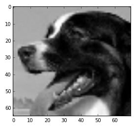
The output from this call tells you that the image type is a numpy.ndarray and that the image size is 90 pixels by 90 pixels. The image is actually an array of pixels that you can manipulate in various ways. For example, if you want to crop the image, you can use the following code to manipulate the image array:
image2 = image[5:70,0:70]
plt.imshow(image2, cmap=cm.gray)
plt.show()
The numpy.ndarray in image2 is smaller than the one in image, so the output is smaller as well. The example below shows typical results. The purpose of cropping the image is to make it a specific size. Both images must be the same size for you to analyze them. Cropping is one way to ensure that the images are the correct size for analysis.
Another method that you can use to change the image size is to resize it. The following code resizes the image to a specific size for analysis:
image3 = resize(image2, (30, 30), mode='nearest')
plt.imshow(image3, cmap=cm.gray)
print("data type: %s, shape: %s" %
(type(image3), image3.shape))
The output from the print() function tells you that the image is now 30 pixels by 30 pixels in size. You can compare it to any image with the same dimensions.
After you have cleaned up all the images and made them the right size, you need to flatten them. A dataset row is always a single dimension, not two or more dimensions. The image is currently an array of 30 pixels by 30 pixels, so you can’t make it part of a dataset. The following code flattens image3, so it becomes an array of 900 elements stored in image_row.
image_row = image3.flatten()
print("data type: %s, shape: %s" %
(type(image_row), image_row.shape))
Notice that the type is still a numpy.ndarray. You can add this array to a dataset and then use the dataset for analysis purposes. The size is 900 elements, as anticipated.