You can find the reduced row echelon form of a matrix to find the solutions to a system of equations. Although this process is complicated, putting a matrix into reduced row echelon form is beneficial because this form of a matrix is unique to each matrix (and that unique matrix could give you the solutions to your system of equations).
The reduced row echelon form of a matrix is a matrix with a very specific set of requirements. These requirements pertain to where any rows of all 0s lie as well as what the first number in any row is. Note: The first number in a row of a matrix that is not 0 is called the leading coefficient. To be considered to be in reduced row echelon form, a matrix must meet all the following requirements:
All rows containing all 0s are at the bottom of the matrix.
All leading coefficients are 1.
Any element above or below a leading coefficient is 0.
The leading coefficient of any row is always to the left of the leading coefficient of the row below it.
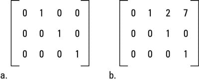 A matrix (a) in reduced row echelon form and (b) not in reduced row echelon form.
Figure a shows you a matrix in reduced row echelon form, and Figure b is not in reduced row echelon form because the 7 is directly above the leading coefficient of the last row and the 2 is above the leading coefficient in row two.
The reduced row echelon form of a matrix comes in handy for solving systems of equations that are 4 x 4 or larger, because the method of elimination would entail an enormous amount of work on your part. The following example shows you how to get a matrix into reduced row echelon form using elementary row operations. You can use any of these operations to get a matrix into reduced row echelon form:
Multiply each element in a single row by a constant (other than zero).
Interchange two rows.
Add two rows together.
Using these elementary row operations, you can rewrite any matrix so that the solutions to the system that the matrix represents become apparent.
Use the reduced row echelon form only if you’re specifically told to do so by a pre-calculus teacher or textbook. Reduced row echelon form takes a lot of time, energy, and precision. It can take a lot of steps, which means that you can get mixed up in tons of places. If you have the choice, you should opt for a less rigorous tactic (unless, of course, you’re trying to show off).
Perhaps the most famous (and useful) matrix in pre-calculus is the identity matrix, which has 1s along the diagonal from the upper-left corner to the lower-right and has 0s everywhere else. It is a square matrix in reduced row echelon form and stands for the identity element of multiplication in the world of matrices, meaning that multiplying a matrix by the identity results in the same matrix.
The identity matrix is an important idea in solving systems because if you can manipulate the coefficient matrix to look like the identity matrix (using legal matrix operations), then the solution to the system is on the other side of the equal sign.
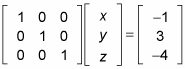
Rewriting this matrix as a system produces the values x = –1, y = 3, and z = –4.
But you don’t have to take the coefficient matrix this far just to get a solution. You can write it in row echelon form, as follows:
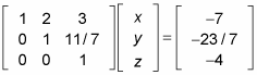
This setup is different from reduced row echelon form because row echelon form allows numbers to be above the leading coefficients but not below.
Rewriting this system gives you the following from the rows:
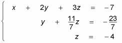
How do you get to the solution — the values of x, y, and z — from there? The answer to that question is back solving, also known as back substitution. If a matrix is written in row echelon form, then the variable on the bottom row has been solved for (as z is here). You can plug this value into the equation above to solve for another variable and continue this process, moving your way up (or backward) until you have solved for all the variables. As with a system of equations, you move from the simplest equation to the most complicated.
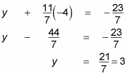
Here’s how you execute the back solving: Now that you know z = –4, you can substitute that value into the second equation to get y:
And now that you know z and y, you can go back further into the first equation to get x:
x + 2(3) + 3(–4) = –7
x + 6 – 12 = –7
x – 6 = –7
x = –1