Probit and logit functions are both nonlinear in parameters, so ordinary least squares (OLS) can’t be used to estimate the betas. Instead, you have to use a technique known as maximum likelihood (ML) estimation.
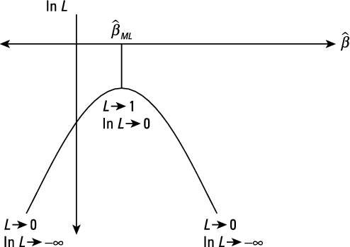
The objective of maximum likelihood (ML) estimation is to choose values for the estimated parameters (betas) that would maximize the probability of observing the Y values in the sample with the given X values. This probability is summarized in what is called the likelihood function.
Constructing the likelihood function
The likelihood function, which calculates the joint probability of observing all the values of the dependent variable, assumes that each observation is drawn randomly and independently from the population. If the values of the dependent variable are random and independent, then you can find the joint probability of observing all the values simultaneously by multiplying the individual density functions.
Assuming that each observed value of the dependent variable is random and independent, the likelihood function is
where pi is the product (multiplication) operator. You can rewrite this equation as
where P represents the probability that Y = 1, (1 – P) is the probability that Y = 0, and F can represent that standard normal or logistic CDF; in the probit and logit models, these are the assumed probability distributions.
The log transformation and ML estimates
In order to make the likelihood function more manageable, the optimization is performed using a natural log transformation of the likelihood function. You can justify it mathematically because log transformations are a type of monotonic transformation. In other words, for any function f(X) and log transformation
Therefore, the optimizing solution for the likelihood function is the same as the log likelihood function.
From the likelihood function L, using a natural log transformation you can write the estimated log likelihood function as
where F denotes either the standard normal CDF (for the probit model) or the logistic CDF (for the logit model). Finding the optimal values for the
terms requires solving the following first-order conditions
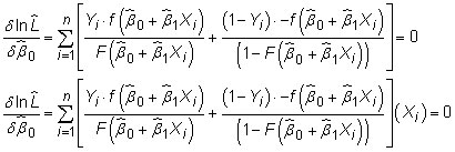
ML estimation is computationally intense because the first-order conditions for maximization don’t have a simple algebraic representation. Econometric software relies on numerical optimization by searching for the values of the
that achieve the largest possible value of the log likelihood function, which means that a process of iteration (a repeated sequence of gradually improving solutions) is required to estimate the coefficients.
The econometric software searches (uses an iterative process) until it finds the values for all the
that simultaneously maximize the likelihood of obtaining the observed values of the dependent variable.