


Make sure the AutoFilter is turned off.
Click the Filter button on the Data tab, if necessary.
Select the first four rows of the worksheet.
This is where you will insert the criteria range.
Right-click the selected rows and choose Insert.
Your table moves down four rows, and you get four empty rows to work with.
Select the header row in the table, and click the Copy button on the Home tab.
A marquee appears around the copied area.
Click cell A1, and then click the Paste button on the Home tab.
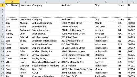
This copies the header row of your table to the first blank row in the worksheet. You now have a criteria range ready to enter filter selections.
In the first blank row of the criteria range, enter the data you want to match.
For example, if you want to locate any entries for the state of Indiana, type IN directly under the State heading.
Enter any additional filter criteria.
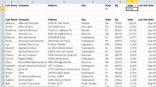
If you want Excel to find data that meets more than one restriction, enter the additional criteria in another field on the first criteria row. This is called an AND filter. If you want Excel to find data that meets at least one of the criteria (an OR filter), enter the filter data on the second row of the criteria range.
Click any cell in the main part of the table.
You shouldn’t have any of your filter criteria selected before you begin the next step.
Click the Advanced button in the Sort & Filter group of the Data tab.
Excel displays the Advanced Filter dialog box.
Select the Filter the List, In-Place option in the Action section.
If you want the filter results to appear in another location in the current worksheet, select Copy to Another Location instead (and then specify the location in the Copy To text box).
Verify the table range in the List Range box.
Make sure Excel recognizes the entire table.
Specify the criteria range including the header row, but not any blank rows.
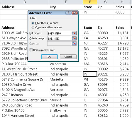
You can type the range address or drag to select the range in the worksheet. Be sure to specify only the rows that contain filtering information. If you include blank rows in your criteria range, Excel includes them in the filtering process. The effect is that no data is filtered out, so all records are returned.
Click OK to display the search results.
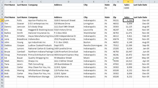
The tables displays the filtered results. The records that don’t fit the criteria are hidden.
When you’re ready to view all data records again, click the Clear button on the Data tab.
All the hidden records reappear.

