


You can see a normal distribution’s shape in this figure.
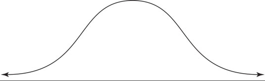 Laypeople call it a bell curve; you call it a normal distribution.
Every normal distribution has certain properties. You can use these properties to determine the relative standing of any particular result on the distribution.
When you understand the properties of the normal distribution, you'll find it easier to interpret statistical data. A continuous random variable X has a normal distribution if its values fall into a smooth (continuous) curve with a bell-shaped pattern. Each normal distribution has its own mean, denoted by the Greek letter μ and its own standard deviation, denoted by the Greek letter σ.
But no matter what their means and standard deviations are, all normal distributions have the same basic bell shape.
The properties of any normal distribution (bell curve) are as follows:
- The shape is symmetric.
- The distribution has a mound in the middle, with tails going down to the left and right.
- The mean is directly in the middle of the distribution. (The mean of the population is designated by the Greek letter μ.)
- The mean and the median are the same value because of the symmetry.
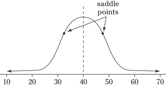
- The standard deviation is the distance from the center to the saddle point (the place where the curve changes from an “upside-down-bowl” shape to a “right-side-up-bowl” shape. (The standard deviation of the population is designated by the Greek letter σ.)
- About 68 percent of the values lie within one standard deviation of the mean, about 95 percent lie within two standard deviations, and most of the values (99.7 percent or more) lie within three standard deviations by the empirical rule.
- Each normal distribution has a different mean and standard deviation that make it look a little different from the rest, yet they all have the same bell shape.
Take a look at the following figure.

Finally, Examples (b) and (c) have different means and different standard deviations entirely; Example (b) has a higher mean which shifts the graph to the right, and Example (c) has a smaller standard deviation; its data values are the most concentrated around the mean.
Note that the mean and standard deviation are important in order to properly interpret numbers located on a particular normal distribution. For example, you can compare where the value 120 falls on each of the normal distributions in the above figure. In Example (a), the value 120 is one standard deviation above the mean (because the standard deviation is 30, you get 90 + 1[30> = 120). So on this first distribution, the value 120 is the upper value for the range where the middle 68% of the data are located, according to the Empirical Rule.
In Example (b), the value 120 lies directly on the mean, where the values are most concentrated. In Example (c), the value 120 is way out on the rightmost fringe, 3 standard deviations above the mean (because the standard deviation this time is 10, you get 90 + 3[10> = 120). In Example (c), values beyond 120 are very unlikely to occur because they are beyond the range where the middle 99.7% of the values should be, according to the Empirical Rule.
