


If your outcome of interest is qualitative, you use a dummy dependent variable and estimate the probability that the outcome (Y = 1) occurs using your econometric model. Although OLS can be used to estimate a model with a qualitative dependent variable, doing so would result in an error term that’s heteroskedastic and isn’t normally distributed.
The most obvious problem with estimating a dummy dependent variable model using OLS is that the predicted probabilities aren’t guaranteed to be within the [0,1] interval. OLS can’t be modified to fully address this issue because nonlinearity in parameters is required in order to guarantee that all predicted probabilities have sensible values. Consequently, an alternative specification must be used. Econometricians choose either the probit or the logit function.
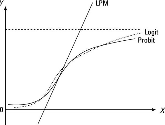
With a probit or logit function, the conditional probabilities are nonlinearly related to the independent variable(s). Additionally, both functions have the characteristic of approaching 0 and 1 gradually (asymptotically), so the predicted probabilities are always sensible.
The figure illustrates the conditional probabilities from an OLS (also known as the linear probability model LPM), a probit, and a logit model.
Working from the standard normal CDF: The probit model
The probit model is based on the standard normal cumulative density function (CDF), which is defined as
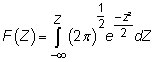
where Z is a standardized normal variable and e is the base of the natural log (the value 2.71828 . . .).
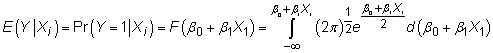
In a probit model, the standard normal CDF replaces the linear function, so you estimate
The beta terms can’t be estimated using OLS, so you need to use a technique known as maximum likelihood (ML).
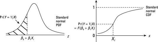
For any given X, the probit model provides the Z value for the observation. The standard normal PDF or CDF can then be used to obtain the probability that Y = 1 for that observation.
The following figure shows how to go about finding the probability for any given observation.
After estimating a probit model, most econometric software can calculate the predicted probabilities for all sample observations.
Basing off of the logistic CDF: The logit model
The logit model is based on the logistic cumulative density function (CDF), defined as
where G is a logistic random variable and e is the base of the natural log (the value 2.71828 . . .).
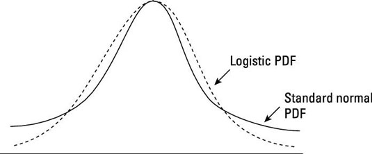
The logistic distribution may be unfamiliar to you, but it’s similar to a standard normal. However, it does have less density within one standard deviation of the mean than a standard normal distribution. The following figure illustrates the difference between the standard normal and the logistic distributions.
In a logit model, the logistic CDF replaces the linear function so that you estimate
Note: You can’t use OLS to estimate the betas; instead, you have to use the maximum likelihood (ML) technique.
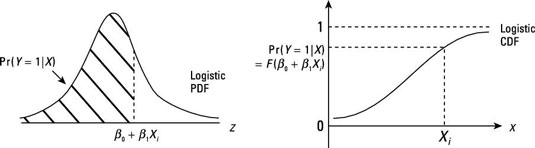
For any given X, the logit model provides the value for the observation that can be used with the logistic CDF to find the probability that Y = 1 for that observation.
The following figure illustrates how you find the probability for any given observation.
When you have your logit model estimated, you can use econometric software such as STATA to calculate the predicted probabilities for all your sample observations.

