
You’re given the task of designing an analog (continuous-time) filter to meet the amplitude response specifications shown. You also need to find the filter step response, determine the value of the peak overshoot, and time where the peak overshoot occurs.
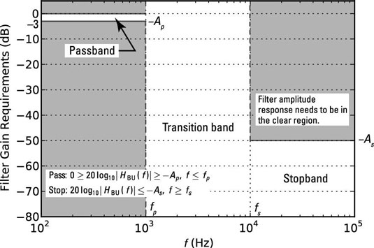
The objective of the filter design is for the frequency response magnitude in dB (20log10|H(f)|) to pass through the unshaded region of the figure as frequency increases. The design requirements reduce to the passband and stopband critical frequencies fp and fs Hz and the passband and stopband attenuation levels Ap and As dB.
Additionally, the response characteristic is to be Butterworth, which means that the filter magnitude response and system function take this form:
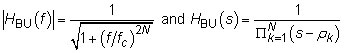
Here, N is the filter order, fc is the passband 3 dB cutoff frequency of the filter, and the poles, located on a semicircle is the left-half s-plane, are given by
This problem requires you to work in the frequency domain, the time domain, and perhaps the s-domain, depending on the solution approach you choose.
From the requirements, the filter frequency response has unity gain (0 dB) in the passband. The step response (a time-domain characterization) of the Butterworth filter is known to overshoot unity before finally settling to unity as
To design the filter, you can use one of two approaches:
Work a solution by hand, using the Butterworth magnitude frequency response |HBU(f)| and the system function, HBU(s).
Use the filter design capabilities of the SciPy signal package.
Finding the filter order and 3 dB cutoff frequency
Follow these steps to design the filter by using Python and SciPy to do the actual number crunching:
Find N and fc to meet the magnitude response requirements.
Use the SciPy function N,wc=signal.buttord(wp,ws,Ap,As,analog= 1) and enter the filter design requirements, where wp and ws are the passband and stopband critical frequencies in rad/s and Ap and As are the passband and stopband attenuation levels (both sets of numbers come from the preceding figure). The function returns the filter order N and the cutoff frequency wc in rad/s.
Synthesize the filter — find the {bk} and {ak} coefficients of the LCC differential equation that realizes the desired system.
If finding circuit elements is the end game, you may go there immediately, using circuit synthesis formulas. Call the SciPy function b,a=signal.butter(N,wc,analog=1) with the filter order and the cutoff frequency, and it returns the filter coefficients in arrays b and a.
Find the step response in exact mathematical form or via simulation.
Here’s how to use the Python tools with the given design requirements and then check the work by plotting the frequency response as an overlay. Note: You can do the same thing in MATLAB with almost the same syntax.
In [<b>379</b>]: N,wc =signal.buttord(2*pi*1e3,2*pi*10e3,3.0,
 50,analog=1) # find filter order N
In [<b>380</b>]: N # filter order
Out[<b>380</b>]: 3
In [<b>381</b>]: wc # cutoff freq in rad/s
Out[<b>381</b>]: 9222.4701630595955
In [<b>382</b>]: b,a = signal.butter(N,wc,analog=1) # get coeffs.
In [<b>383</b>]: b
Out[<b>383</b>]: array([7.84407571e+11+0.j])
In [<b>384</b>]: real(a)
Out[<b>384</b>]: array([1.00000000e+00, 1.84449403e+04,
           1.70107912e+08,7.84407571e+11])
The results of Line [379] tell you that the required filter order is N = 3 and the required filter cutoff frequency is
The filter coefficient sets are also included in the results.
Use the real() function to safely display the real part of the coefficients array a because you know the coefficients are real. How? The poles, denominator roots of HBU(s), are real or occur in complex conjugate pairs, ensuring that the denominator polynomial has real coefficients when multiplied out. The very small imaginary parts are due to numerical precision errors.
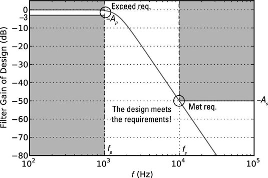
Checking the final design frequency response
To check the design, use the frequency response recipe.
In [<b>386</b>]: f = logspace(2,5,500) # log frequency axis
In [<b>387</b>]: w,H = signal.freqs(b,a,2*pi*f)
In [<b>388</b>]: semilogx(f,20*log10(abs(H)),’g’)
The figure shows the plot of the final design magnitude response along with the original design requirements.
Finding the step response from the filter coefficients
The most elegant approach to finding the step response from the filter coefficients is to find
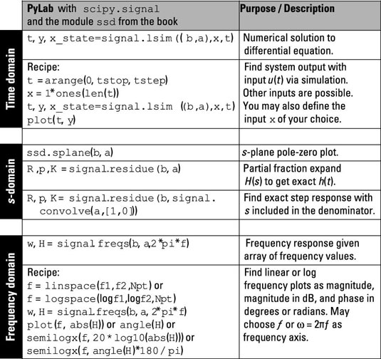
The s-domain section of the figure tells you how to complete the partial fraction expansion (PFE) numerically. You have the coefficient arrays for H(s), so all you need to do is multiply the denominator polynomial by s. You can do this by hand or you can use a relationship between polynomial coefficients and sequence convolution.
When you multiply two polynomials, the coefficient arrays for each polynomial are convolved, as in sequence convolution.
Here, you work through the problem, using signal.convolve to perform polynomial multiplication in the denominator. To convince you that this really works, consider multiplication of the following two polynomials:
(x2 + x + 1)(x + 1) = x3 + 2x2 + 2x + 1
If you convolve the coefficients sets [1, 1, 1] and [1, 1] as arrays in Python, you get this output:
In [<b>418</b>]: signal.convolve([1,1,1],[1,1])
Out[<b>418</b>]: array([1, 2, 2, 1])
This agrees with the hand calculation. To find the PFE, plug the coefficients arrays b and convolve(a,[1,0]) into R,p,K = residue(b,a). The coefficients [1, 0] correspond to the s-domain polynomial s + 0.
In [<b>420</b>]: R,p,K = signal.residue(b,signal.convolve([1,0],a))
In [<b>421</b>]: R #(residues) scratch tiny numerical errors
Out[<b>421</b>]:
array([ 1.0000e+00 +2.3343e-16j, # residue 0, imag part 0
 -1.0000e+00 +1.0695e-15j, # residue 1, imag part 0
 1.08935e-15 -5.7735e-01j, # residue 2, real part 0
 1.6081e-15 +5.7735e-01j]) # residue 3, real part 0
In [<b>422</b>]: p #(poles)
Out[<b>422</b>]:
array([ 0.0000 +0.0000e+00j, # pole 0
 -9222.4702 -1.5454e-12j, # pole 1, imag part 0
 -4611.2351 -7.9869e+03j, # pole 2
 -4611.2351 +7.9869e+03j])# pole 3
In [<b>423</b>]: K #(from long division)
Out[<b>423</b>]: array([ 0.+0.j]) # proper rational, so no terms
You have four poles: two real and one complex conjugate pair — a bit of a mess to work through, but it’s doable. Refer to the transform pair
to calculate the inverse transform for all four terms.
For the conjugate poles, the residues are also conjugates. This property always holds.
You can write the inverse transform of the conjugate pole terms as sines and cosines, using Euler’s formula and the cancellation of the imaginary parts in front of the cosine and real parts in front of the sine:
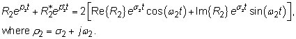
Putting it all together, you get ystep(t) = u(t) – e–9,222.47tu(t)–2 x 0.5774e–4,611.74tsin(7,986.89t)u(t). Having this form is nice, but you still need to find the function maximum for t > 0 and the maximum location. To do this, plot the function and observe the maximum.
A more direct approach is to use simulation via signal.lsim and the time-domain recipe. The system input is a step, so the simulation output will be the step response. From the simulated step response, you can calculate the peak overshoot numerically and see it in a plot. The IPython command line code is
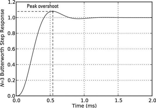
In [<b>425</b>]: t = arange(0,0.002,1e-6) # step less than smallest time constant
In [<b>426</b>]: t,ys,x_state = signal.lsim((b,a),ones(len(t)),t)
In [<b>428</b>]: plot(t*1e3,ys)
Using the time array t and the step response array ys, you can use the max() and find() functions to complete the task:
In [<b>436</b>]: max(real(ys)) # real to clear num. errors
Out[<b>436</b>]: 1.0814651457627822 # peak overshoot is8.14%
In [<b>437</b>]: find(real(ys)== max(real(ys)))
Out[<b>437</b>]: array([534]) # find peak to be at index 534
In [<b>439</b>]: t[534]*1e3 # time at index 534 in ms
Out[<b>439</b>]: 0.5339