


Most economic time series grow over time, but sometimes time series actually decline over time. In either case, you’re looking at a time trend. The most common models capturing time trends are either linear or exponential.
If the dependent variable has a relatively steady increase over time, your best bet is to model the relationship with a linear time trend. However, if the growth rate is fairly steady (while the rate at which the value of the dependent variable changes isn’t constant), then you need to model the relationship with an exponential time trend.
A linear time trend has the form

where t is the time trend variable (usually a sequential numbering of the time periods beginning with a value of 1) and

is the time trend coefficient and represents the rate at which the value of the dependent variable changes, on average, in each subsequent time period. If the time trend coefficient is positive, then the dependent variable increases over time. If the time trend coefficient is negative, then the dependent variable decreases over time.
You can express an exponential time trend as

where t is the time trend variable and
is the time trend coefficient and represents the rate at which the growth of the dependent variable changes, on average, in each subsequent time period. If the time trend coefficient is positive, then the dependent variable’s growth rate is positive over time. If the time trend coefficient is negative, then the dependent variable’s growth rate is negative over time.
The figure shows a STATA graph of yearly inventories from 1950 to 1991 and an estimated time trend model. Most datasets don’t contain a time variable, so you can sort the data using the variable that captures the sequencing of observations (year) and create the time variable.
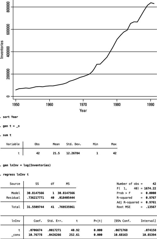
Given the depiction of the time series, applying the exponential time trend model is most appropriate in this case. The estimated value of 0.07 for
implies that, on average, inventories have grown at a rate of approximately 7 percent per year.
In the example, creating the trend variable is a straightforward procedure because there’s only one time variable. But in some cases, multiple time variables exist. For example, with monthly data that spans several years, the data is likely to contain a year and month variable. In that case, you’d want to sort by both year and month before you create the trend variable.
When dealing with observations measured over multiple time periods, the value of the trend variable should always represent the order of the observation in a chronological sequence.
If you’d like to avoid using a log transformation of your dependent variable (perhaps it doesn’t seem appropriate with the other factors that you’ve included in the model as independent variables), then a quadratic time trend can also work well in situations where the time trend isn’t linear.
Although higher order polynomials could be used for your time trend, they aren’t popular among applied econometricians because they’re difficult to justify theoretically and typically consume additional degrees of freedom without significantly increasing the explanatory power.

