Determining price through demand and supply
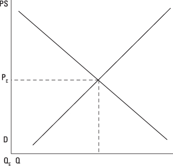
Markets move to a price that equates the quantity of a good consumers are willing and able to purchase (the quantity demanded) with the quantity of the good firms are willing to provide (the quantity supplied). When markets reach the point where quantity demanded equals quantity supplied, they’re in equilibrium.
At this point, all buyers and sellers are satisfied: Everyone who wants to buy the good at the equilibrium price can buy it, and everyone who wants to sell the good at the equilibrium price can sell it. Equilibrium corresponds to the intersection of the demand and supply curves. At that point, the equilibrium price corresponds to PE, and the equilibrium quantity corresponds to QE as illustrated in the figure.
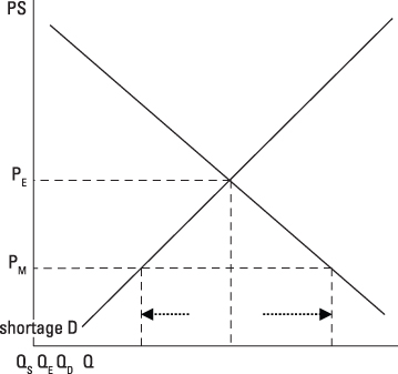
If the market initially has a price below the equilibrium price, such as PM in the following figure, the market has a shortage. Consumers want to buy a greater quantity of the good than businesses are willing to provide. In other words, quantity demanded, QD, is greater than quantity supplied, QS.
The shortage equals the difference between the quantity demanded and the quantity supplied. When a shortage exists, consumers who want the good but can’t buy it offer a higher price, so the market price rises toward equilibrium. When the market price finally reaches equilibrium, the shortage entirely disappears.
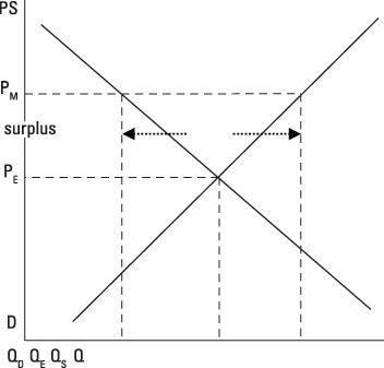
Similarly, if the market initially has a price that is above the equilibrium price, the market has a surplus. Businesses want to sell a greater quantity of the good than consumers want to buy, so the quantity supplied, QS, is greater than the quantity demanded, QD.
The surplus is the difference between the quantity supplied and the quantity demanded. When a surplus exists, businesses lower the price to sell their accumulating inventory — the items they can’t sell at the high price. The market price falls toward equilibrium, and when it finally reaches equilibrium, the surplus disappears.
Maximizing profit with marginal revenue and marginal cost
Profit equals total revenue minus total cost. Given businesses want to maximize profit, they should keep producing more output as long as an additional unit adds more to revenue than it adds to cost. Economists call the added revenue marginal revenue and the added cost marginal cost. Thus, firms should continue producing more output until marginal revenue equals marginal cost. That’s the point where profits are maximized.
Marginal revenue can be a little tricky. In order to sell more output, firms frequently have to lower price. This lower price means the firm gets less revenue not only for the last unit, but all other units produced, because firms usually charge the same price for every unit they sell.
In this situation, the last unit’s marginal revenue equals its price minus the decrease in revenue that occurs because a lower price is charged for every other unit. The crucial point you need to remember is that marginal revenue in this situation is less than price.
Marginal revenue and marginal cost can be determined with calculus. Because marginal revenue is the change in total revenue that occurs when an additional unit of output is produced and sold, marginal revenue is the derivative of total revenue taken with respect to quantity.
Similarly, marginal cost is the change in total cost that occurs when one additional unit of a good is produced, so it’s the derivative of total cost taken with respect to quantity. You can determine the profit-maximizing quantity of output by setting these two derivatives equal to one another.
Responding to the price elasticity of demand
Elasticity measures how responsive quantity is to a change in another variable. For example, the price elasticity of demand measures the responsiveness of quantity demanded to a change in the good’s price.
The price elasticity of demand, η, for a segment of the demand curve is calculated using the following formula:
In the formula, P0 and Q0 represent the initial or starting price/quantity combination, and P1 and Q1 represent the ending price/quantity combination.
Once calculated, the price elasticity of demand indicates how responsive quantity demanded is to a change in the good’s price:
-
Perfectly inelastic: The price elasticity of demand equals zero, indicating that quantity demanded doesn’t change in response to a change in the good’s price.
-
Inelastic: The price elasticity of demand is between –1 and 0, indicating that quantity demanded isn’t very responsive to a change in the good’s price.
-
Unitary elastic: The price elasticity of demand equals –1, indicating the percentage change in quantity demanded equals the percentage change in price.
-
Elastic: The price elasticity of demand is less than –1, indicating that quantity demanded is very responsive to a change in the good’s price.
-
Perfectly elastic: If demand is perfectly elastic, the demand curve is a horizontal line instead of the usual downward-sloping demand curve.
Once calculated, the price elasticity of demand is used to determine the relationship between price changes and changes in total revenue. If demand is inelastic, price and total revenue are directly related, so increasing price increases total revenue. If demand is elastic, price and total revenue are inversely related, so increasing price decreases total revenue.
Calculating the time value of money
Calculating the time value of money is important. Basically, as long as you can earn interest, you’d rather have a dollar today instead of a dollar one year from now. If you receive that dollar today and the interest rate is 5 percent, one year from now you’ll have $1.05, and that’s certainly better than a dollar. This idea becomes even more important for businesses when thousands or millions of dollars are involved.
Many business decisions involve investing money today in order to get some amount of future profit. Because you’re receiving the money/profit in the future, you need to discount it because you can’t use it today to earn interest. This discounting is accomplished by calculating the present value of the money you receive in the future.
Present value (PV) is determined through the following formula:
Because profit equals revenue minus cost, the numerator of this calculation represents profit for some future year (t) — year t’s revenue (Rt,) minus year t’s cost (Ct). The denominator is 1 plus the interest rate (R) expressed in decimal form: 5 percent interest is 0.05. The power used in the denominator is how many year’s into the future you receive the money — three years into the future means t equals 3. And, because you’re likely to receive this profit for more than one year, you determine this value for each year and then add or sum up all the values.
Determining the cost of capital
Investing in factories, machinery, and equipment — capital — requires money. Those funds can be borrowed (external equity), or the business can raise the funds internally, equity either from the firm’s or the owner’s financial resources.
The cost of using external equity or debt capital is the interest rate you pay lenders. However, because interest expenses are tax deductible, the after tax cost of debt (kd) is the interest rate (r) multiplied by 1 minus the firm’s marginal tax rate (t) or
Internal equity from the firm or the firm’s owners also has a cost. The opportunity cost of funds you invest in the firm is the interest you could have earned if you invested those funds elsewhere. You can choose from among three alternatives to determine the cost of internal or equity capital.
-
Risk premium method: The risk premium method assumes that you incur some additional risk in the investment. This method’s cost estimation uses a risk-free rate of return, rf, plus an additional risk premium, rp, or

where ke is the cost of equity capital. The U.S. Treasury Bill rate is often used as the risk-free rate of return.
-
Dividend valuation method: The dividend valuation method is based on shareholder attitudes. A shareholder’s rate of return equals the dividend (D) divided by the stock price per share (P), plus any expected earnings growth (g). Using this shareholder return as the cost of equity capital results in

-
Capital asset pricing method: The final method for determining the cost of internal equity is the capital-asset-pricing method. This method incorporates a risk premium for variability in a company’s return — stocks with greater variability in return have higher risk premiums. The cost of internal equity using the capital-asset-pricing method is
where rf is the risk free return, km is an average stock’s return, and β measures the variability in the specific firm’s common stock return relative to the variability in the average stock’s return. If β equals 1, the firm has average variability or risk. β values greater than 1 indicate higher than average variability or risk, while values less than 1 indicate below-average risk. The term β(km – rf) gives the risk premium for holding the firm’s common stock.
Many firms finance capital investment with a combination of external and internal funds. The composite cost of capital (kc) is a weighted average of the cost of internal equity and the cost of external or debt equity. In the following equation
we and wd are the weights or proportions of internal equity and debt you use to finance the project.