
Here is a detailed analytical solution to a convolution integral problem, followed by detailed numerical verification, using PyLab from the IPython interactive shell (the QT version in particular). The intent of the numerical solution is to demonstrate how computer tools can verify analytical solutions to convolution problems.
Set up PyLab
To get started with PyLab and the IPython interactive shell, you can readily set up the tools on Mac OS, Windows, and Ubuntu Linux.
Setting up on Ubuntu Linux is perhaps the easiest because you can just use the Ubuntu Software Center. On Mac and Windows OS, you can use a monolithic installation, which installs most everything you need all at once. Check out the free version from Enthought, but others are available on the web.
Verify continuous-time convolution
Here is a convolution example employing finite extent signals. Full analytical solutions are included, but the focus is on numerical verification, in particular, using PyLab and the freely available custom code module ssd.py mentioned earlier.
Consider the convolution integral for two continuous-time signals x(t) and h(t) shown.
![[Credit: Illustration by Mark Wickert, PhD]](https://www.dummies.com/wp-content/uploads/378841.image0.jpg)
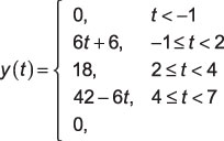
To arrive at the analytical solution, you need to break the problem down into five cases, or intervals of time t where you can evaluate the integral to form a piecewise contiguous solution. When you put these five contiguous intervals together, you have a complete solution for all values of t:
From the study of convolution integrals, you discover that you can write the support or active interval for the output y(t) in terms of the support intervals for each of the input signals. That result states that the output support interval runs from the sum of the starting values for x(t) and h(t) and ends at the ending values. Thus, the support interval for y(t) is at most
In this example, each case is treat as a step in the solution that follows:
Case 1: You start with t + 1 < 0, or equivalently t < –1. The product of waveforms h(λ) and x(t – λ) don’t overlap in the convolution integral integrand, so for Case 1 the integral is just y(t) = 0 for t < –1.
Case 2: Consider the next interval to the right of Case 1. This case is formed by the joint condition of the signal edge at t + 1 ≥ 0 and t + 1 < 3, which is equivalent to writing –1 ≤ t < 2. The integrand of the convolution integral is 2 x 3 with the integration limits running from 0 to t + 1.
You find y(t) on this interval by evaluating the convolution integral:

Case 3: The next interval in the series is t + 1 ≥ 3 and t – 4 < 0 or 2 ≤ t < 4. The integrand is again 2 x 3, but now the integration limits run from 0 to 3. Evaluating the convolution integral yields the following:

Case 4: The final interval involving signal overlap occurs when t – 4 ≥ 0 and t – 4 < 3, which implies that 4 ≤ t ≤ 7. The integration limits run from t – 4 to 3, so the convolution integral result is

Case 5: You can see that when t – 4 > 3 or t > 7, no overlap occurs between the signals of the integrand, so the output is y(t) = 0, t > 7.
Collecting the various pieces of the solution, you have the following:
Verifying this solution with Python involves two steps: (1) plotting the analytical solution and (2) comparing it with the plot of the numerical solution, using functions found in the code module ssd.py. Here are the details for completing these steps:
Create a piecewise function in Python that you can then evaluate over a user-defined range of time values.
You can write this function right in the IPython shell as shown here:
In [<b>68</b>]: def pulse_conv(t):
    ...: y = zeros(len(t)) # initialize output array
    ...: for k,tk in enumerate(t): # make y(t) values
    ...:     if tk >= -1 and tk < 2:
    ...:          y[k] = 6*tk + 6
    ...:     elif tk >= 2 and tk < 4:
    ...:          y[k] = 18
    ...:     elif tk >= 4 and tk <= 7:
    ...:          y[k] = 42 - 6*tk
    ...: return y
Note that the Python language is sensitive to indents, so pay attention to the indents when entering this code into IPython. The good news is that IPython understands the needs of Python and does a good job of indenting code block automatically.
Numerically evaluate the convolution by first creating representations of the actual waveforms of the convolution and then performing the numerical convolution.
To get access to the functions in the module ssd.py, you need to import the module in your IPython session, using In [69]: import ssd.
Then you can access the functions in the module by using the namespace prefix ssd. The function y, ny = ssd.conv_integral(x1, tx1, x2, tx2, extent=('f', 'f')) performs the actual convolution.
You load time sampled versions of the signals to be convolved into the arguments x1 and x2, with tx1 and tx2 being the corresponding time axes. All four of these variables are NumPy ndarrays. The function returns the convolution result y followed by ny, as a Python tuple. The rectangular pulse shapes are created with the function ssd.rect(n,tau) and time axis shifting in the function arguments.
Putting it all together, the code for numerically approximating the convolution integral output is as follows (only critical code statements shown):
In [<b>89</b>]: t = arange(-8,9,.01)
In [<b>90</b>]: xc1 = 2*ssd.rect(t-1.5,5)
In [<b>91</b>]: hc1 = 3*ssd.rect(t-1.5,3)
In [<b>93</b>]: subplot(211)
In [<b>94</b>]: plot(t,xc1)
In [<b>99</b>]: subplot(212)
In [<b>100</b>]: plot(t,hc1)
In [<b>101</b>]: savefig('c1_intputs.pdf')
In [<b>115</b>]: yc1_num,tyc1 = ssd.conv_integral(xc1,t,hc1,t)
Output support: (-16.00, +17.98)
In [<b>116</b>]: subplot(211)
In [<b>117</b>]: plot(t,pulse_conv(t))
In [<b>123</b>]: subplot(212)
In [<b>125</b>]: plot(tyc1,yc1_num)
In [<b>130</b>]: savefig('c1_outputs.pdf')
The following figure shows plots of the signals x(t) and h(t).
![[Credit: Illustration by Mark Wickert, PhD]](https://www.dummies.com/wp-content/uploads/378849.image8.jpg) Credit: Illustration by Mark Wickert, PhD
Credit: Illustration by Mark Wickert, PhD
Finally, the numerical representation of y(t) is plotted along with the analytical solution shown.
![[Credit: Illustration by Mark Wickert, PhD]](https://www.dummies.com/wp-content/uploads/378850.image9.jpg)
From a plot perspective, the two solutions agree, so the analytical solution is confirmed.