


When using a test statistic for one population mean, there are two cases where you must use the t-distribution instead of the Z-distribution. The first case is where the sample size is small (below 30 or so), and the second case is when the population standard deviation,
is not known, and you have to estimate it using the sample standard deviation, s. In both cases, you have less reliable information on which to base your conclusions, so you have to pay a penalty for this by using the t-distribution, which has more variability in the tails than a Z-distribution has.
A hypothesis test for a population mean that involves the t-distribution is called a t-test. The formula for the test statistic in this case is:

where tn-1 is a value from the t-distribution with n–1 degrees of freedom.
Note that it is just like the test statistic for the large sample and/or normal distribution case, except
is not known, so you substitute the sample standard deviation, s, instead, and use a t-value rather than a z-value.
Because the t-distribution has fatter tails than the Z-distribution, you get a larger p-value from the t-distribution than one that the standard normal (Z-) distribution would have given you for the same test statistic. A bigger p-value means less chance of rejecting a null hypothesis, H0. Having less data and/or not knowing the population standard deviation should create a higher burden of proof.
Suppose a delivery company claims they deliver their packages in 2 days on average, and you suspect it’s longer than that. The hypotheses are
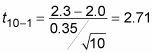
To test this claim, you take a random sample of 10 packages and record their delivery times. You find the sample mean is
and the sample standard deviation is 0.35 days. (Because the population standard deviation,
is unknown, you estimate it with s, the sample standard deviation.) This is a job for the t-test.
Because the sample size is small (n =10 is much less than 30) and the population standard deviation is not known, your test statistic has a t-distribution. Its degrees of freedom is 10 – 1 = 9. The formula for the test statistic (referred to as the t-value) is:
To calculate the p-value, you look in the row in the t-table for df = 9.
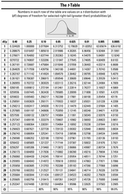
Your test statistic (2.71) falls between two values in the row for df = 9 in the t-table: 2.26 and 2.82 (rounding to two decimal places). To calculate the p-value for your test statistic, find which columns correspond to these two numbers. The number 2.26 appears in the 0.025 column and the number 2.82 appears in the 0.010 column; you now know the p-value for your test statistic lies between 0.025 and 0.010 (that is, 0.010 p-value
Using the t-table you don’t know the exact number for the p-value, but because 0.010 and 0.025 are both less than your significance level of 0.05, you reject H0; you have enough evidence in your sample to say the packages are not being delivered in 2 days, and in fact the average delivery time is more than 2 days.
The temptation is to say, “Well, I knew the claim of 2 days on average was too low because the sample mean of 2.3 minutes was clearly larger. Why do I even need a hypothesis test?” All that number tells you is something about those 10 packages sampled. You also need to factor in variation using the standard error and the t-distribution to be able to say something about the entire population of shipped packages.
The t-table doesn’t include every possible t-value; just find the two values closest to yours on either side, look at the columns they’re in, and report your p-value in relation to theirs. (If your test statistic is greater than all the t-values in the corresponding row of the t-table, just use the last one; your p-value will be less than its probability.)

