


When all else fails, you can use Excel 2013’s Find feature to locate specific information in the worksheet. Choose Home→Find & Select→Find or press Ctrl+F, Shift+F5, or even Alt+HFDF to open the Find and Replace dialog box.
In the Find What drop-down box of this dialog box, enter the text or values you want to locate and then click the Find Next button or press Enter to start the search. Choose the Options button in the Find and Replace dialog box to expand the search options.
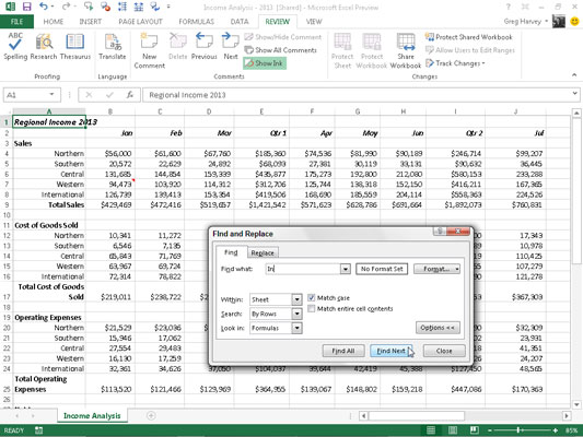
When you search for a text entry with the Find and Replace feature, be mindful of whether the text or number you enter in the Find What text box is separate in its cell or occurs as part of another word or value. For example, if you enter the characters in in the Find What text box and you don’t select the Match Entire Cell Contents check box, Excel finds
The In in Regional Income 2010 in cell A1
The In in International in A8, A16, A24 and so on
The in in Total Operating Expenses in cell A25
If you select the Match Entire Cell Contents box in the Find and Replace dialog box before searching, Excel would not consider the anything in the sheet to be a match because all entries have other text surrounding the text you’re searching for. If you had the abbreviation for Indiana (IN) in a cell by itself and had chosen the Match Entire Cell Contents option, Excel would find that cell.
When you search for text, you can also specify whether you want Excel to match the case you use when entering the search text in the Find What text box. By default, Excel ignores case differences between text in cells of your worksheet and the search text you enter in the Find What text box. To conduct a case-sensitive search, you need to select the Match Case check box.
If the text or values that you want to locate in the worksheet have special formatting, you can specify the formatting to match when conducting the search.
To have Excel match the formatting assigned to a particular cell in the worksheet, follow these steps:
Click the drop-down button on the right of the Format button in the Find and Replace dialog box and choose the Choose Format from Cell option on the pop-up menu.
Excel opens the Find Format dialog box.
Click the Choose Format From Cell button at the bottom of the Find Format dialog box.
The Find Format dialog box disappears, and Excel adds an ink dropper icon to the normal white cross mouse and touch pointer.
Click the ink dropper pointer in the cell in the worksheet that contains the formatting you want to match.
The formatting in the selected worksheet appears in the Preview text box in the Find and Replace dialog box, and you can then search for that formatting in other places in the worksheet by clicking the Find Next button or by pressing Enter.
To select the formatting to match in the search from the options on the Find Format dialog box, follow these steps:
Click the Format button or click its drop-down button and choose Format from its menu.
Select the formatting options to match from the various tabs and click OK.
When you use either of these methods to select the kinds of formatting to match in your search, the No Format Set button changes to a Preview button. The word Preview in this button appears in whatever font and attributes Excel picks up from the sample cell or through your selections in the Find Format dialog box.
To reset the Find and Replace to search across all formats again, click Format→Clear Find Format, and No Form Set will appear again between the Find What and Format buttons.
When you search for values in the worksheet, be mindful of the difference between formulas and values. For example, say cell K24 of your worksheet contains the computed value $15,000. If you type 15000 in the Find What text box and press Enter to search for this value, instead of finding the value 15000 in cell K24, Excel displays an alert box with the following message:
Microsoft Excel cannot find the data you’re searching for
This is because the value in this cell is calculated by the formula
=I24*J24
The value 15000 doesn’t appear in that formula. To have Excel find any entry matching 15000 in the cells of the worksheet, you need to choose Values in the Look In drop-down menu of the Find and Replace dialog box in place of the normally used Formulas option.
If you don’t know the exact spelling of the word or name or the precise value or formula you’re searching for, you can use wildcards, which are symbols that stand for missing or unknown text. Use the question mark (?) to stand for a single unknown character; use the asterisk (*) to stand for any number of missing characters.
Suppose that you enter the following in the Find What text box and choose the Values option in the Look In drop-down menu:
7*4
Excel stops at cells that contain the values 74, 704, and 75,234. Excel even finds the text entry 782 4th Street!
If you actually want to search for an asterisk in the worksheet rather than use the asterisk as a wildcard, precede it with a tilde (~), as follows:
~*4
This arrangement enables you to search the formulas in the worksheet for one that multiplies by the number 4.
The following entry in the Find What text box finds cells that contain Jan, January, June, Janet, and so on.
J?n*

