Moments are summary measures of a probability distribution and include the expected value, variance, and standard deviation. You can use these values to measure to what extent the degrees of freedom affect the F-distribution.
The expected value is known as the first moment of a probability distribution and represents the mean or average value of a distribution.
The variance is the second central moment and shows how spread out or scattered the values of a distribution are around the expected value.
The standard deviation isn’t a separate moment but is the square root of the variance.
For most applications, the standard deviation is more useful than the variance (because the standard deviation is measured in the same units as the expected value whereas the variance is not). For the F-distribution, you use this formula to determine the expected value:
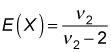
E(X) represents the expected value, and
represents the denominator degrees of freedom.
The expected value formula requires the denominator degrees of freedom to be greater than 2. Otherwise, the expected value becomes negative or undefined.
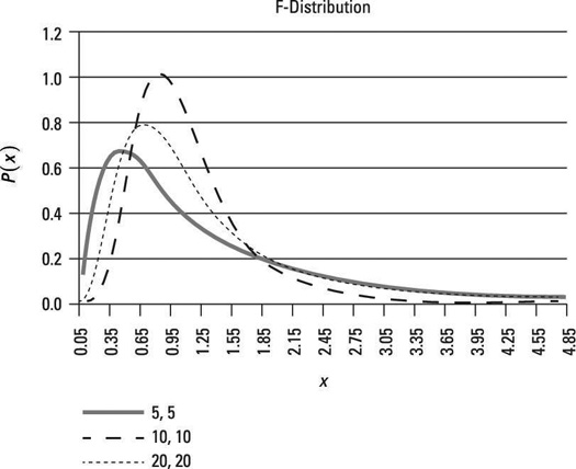
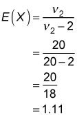
The expected value represents the average value of the F-distribution. For example, this figure shows a graph of the F-distribution with 5 numerator degrees of freedom and 5 denominator degrees of freedom. The expected value equals:
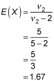
The figure also shows a graph of the F-distribution with 20 numerator degrees of freedom and 20 denominator degrees of freedom. The expected value equals:
This shows that the average value of the F-distribution with 20 numerator degrees of freedom and 20 denominator degrees of freedom is less than the average value of the F-distribution with 5 numerator degrees of freedom and 5 denominator degrees of freedom.
Because both parent populations are normal and have the same variance, and the samples and populations are independent, you know that v1 = n1 – 1 = numerator degrees of freedom, and that v2 = n2 – 1 = denominator degrees of freedom.
To compute the variance, you use this formula:
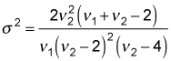
Keep in mind that the variance formula requires the denominator degrees of freedom to be greater than 4; otherwise, the variance becomes negative or undefined.
The standard deviation is the square root of the variance:
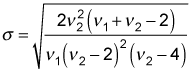
The variance and the standard deviation are used as measures of how spread out the values of the F-distribution are compared with the expected value.
For example, for the F-distribution with 5 numerator degrees of freedom and 5 denominator degrees of freedom, the variance equals
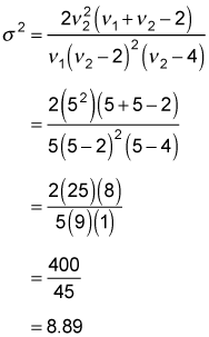
The standard deviation equals the square root of 8.89, or 2.98.
For the F-distribution with 20 numerator degrees of freedom and 20 denominator degrees of freedom, the variance equals
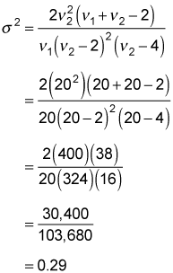
The standard deviation equals the square root of 0.29, or 0.54.
In the figure, the F-distribution with 20 numerator degrees of freedom and 20 denominator degrees of freedom has a tail that falls off very rapidly (so that the distribution is less spread out) compared with the F-distribution with 5 numerator degrees of freedom and 5 denominator degrees of freedom; therefore, the distribution with 20 numerator and denominator degrees of freedom has a lower variance and standard deviation.