
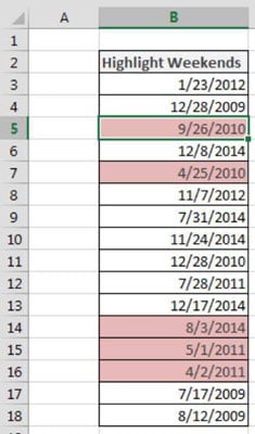
When working with timecards and scheduling in Excel, you often benefit from being able to easily pinpoint any dates that fall on the weekends. The conditional formatting rule illustrated here highlights all the weekend dates in the list of values.
To build this basic formatting rule, follow these steps:
Select the data cells in your target range (cells B3:B18 in this example), click the Home tab of the Excel Ribbon, and then select Conditional Formatting→New Rule.
This opens the New Formatting Rule dialog box.
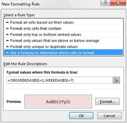
In the list box at the top of the dialog box, click the Use a Formula to Determine which Cells to Format option.
This selection evaluates values based on a formula you specify. If a particular value evaluates to TRUE, the conditional formatting is applied to that cell.
In the formula input box, enter the formula shown with this step.
Note that you use the WEEKDAY function to evaluate the weekday number of the target cell (B3). If the target cell returns as weekday 1 or 7, it means the date in B3 is a weekend date. In this case, the conditional formatting will be applied.
=OR(WEEKDAY(B3)=1,WEEKDAY(B3)=7)
Note that in the formula, you exclude the absolute reference dollar symbols ($) for the target cell (B3). If you click cell B3 instead of typing the cell reference, Excel will automatically make your cell reference absolute. It’s important that you don’t include the absolute reference dollar symbols in your target cell because you need Excel to apply this formatting rule based on each cell’s own value.
Click the Format button.
This opens the Format Cells dialog box, where you have a full set of options for formatting the font, border, and fill for your target cell. After you have completed choosing your formatting options, click the OK button to confirm your changes and return to the New Formatting Rule dialog box.
Back in the New Formatting Rule dialog box, click the OK button to confirm your formatting rule.
If you need to edit your conditional formatting rule, simply place your cursor in any of the data cells within your formatted range and then go to the Home tab and select Conditional Formatting→Manage Rules. This opens the Conditional Formatting Rules Manager dialog box. Click the rule you want to edit and then click the Edit Rule button.